STAT 497 LECTURE NOTE 11 DIAGNOSTIC CHECKS 1

STAT 497 LECTURE NOTE 11 DIAGNOSTIC CHECKS 1

DIAGNOSTIC CHECKS • After identifying and estimating a time series model, the goodness-of-fit of the model and validity of the assumptions should be checked. If we have a perfect model fit, then we can construct the ARIMA forecasts. 2

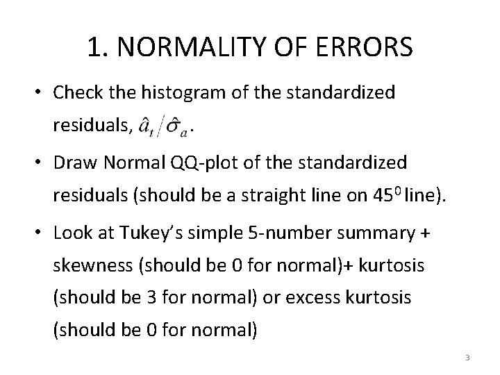
1. NORMALITY OF ERRORS • Check the histogram of the standardized residuals, . • Draw Normal QQ-plot of the standardized residuals (should be a straight line on 450 line). • Look at Tukey’s simple 5 -number summary + skewness (should be 0 for normal)+ kurtosis (should be 3 for normal) or excess kurtosis (should be 0 for normal) 3

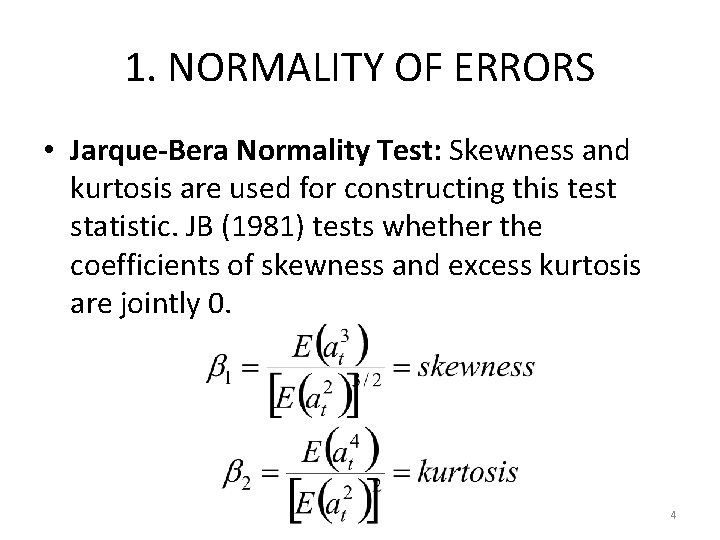
1. NORMALITY OF ERRORS • Jarque-Bera Normality Test: Skewness and kurtosis are used for constructing this test statistic. JB (1981) tests whether the coefficients of skewness and excess kurtosis are jointly 0. 4

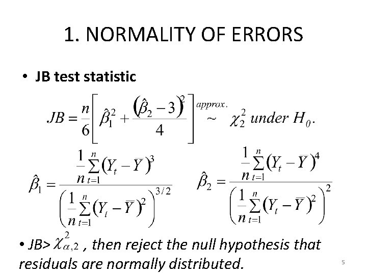
1. NORMALITY OF ERRORS • JB test statistic • JB> , then reject the null hypothesis that residuals are normally distributed. 5

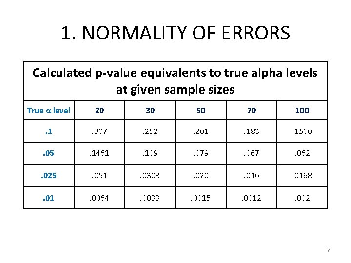
1. NORMALITY OF ERRORS • The chi-square approximation, however, is overly sensitive for small samples, rejecting the null hypothesis often when it is in fact true. Furthermore, the distribution of p-values departs from a uniform distribution and becomes a right-skewed uni-modal distribution, especially for small p-values. This leads to a large Type I error rate. The table below shows some p-values approximated by a chi-square distribution that differ from their true alpha levels for very small samples. • You can also use Shapiro-Wilk test. 6

1. NORMALITY OF ERRORS Calculated p-value equivalents to true alpha levels at given sample sizes True α level 20 30 50 70 100 . 1 . 307 . 252 . 201 . 183 . 1560 . 05 . 1461 . 109 . 079 . 067 . 062 . 025 . 051 . 0303 . 020 . 0168 . 01 . 0064 . 0033 . 0015 . 0012 . 002 7

2. DETECTION OF THE SERIAL CORRELATION • In OLS regression, time residuals are often found to be serially correlated with their own lagged values. • Serial correlation means – OLS is no longer an efficient linear estimator. – Standard errors are incorrect and generally overstated. – OLS estimates are biased and inconsistent if a lagged dependent variable is used as a regressor. 8

2. DETECTION OF THE SERIAL CORRELATION • Durbin-Watson test is for regular regression with independent variables. It is not appropriate for time series models with lagged dependent variables. It only tests for AR(1) errors. There should be a constant term and deterministic independent variables in the model. 9

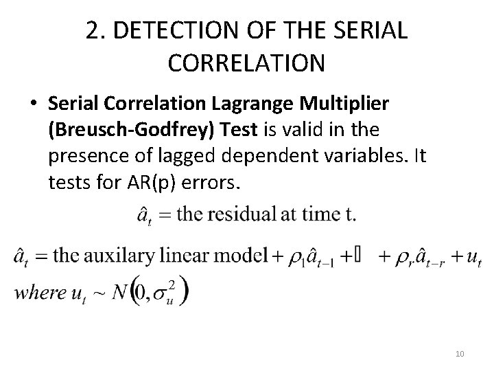
2. DETECTION OF THE SERIAL CORRELATION • Serial Correlation Lagrange Multiplier (Breusch-Godfrey) Test is valid in the presence of lagged dependent variables. It tests for AR(p) errors. 10

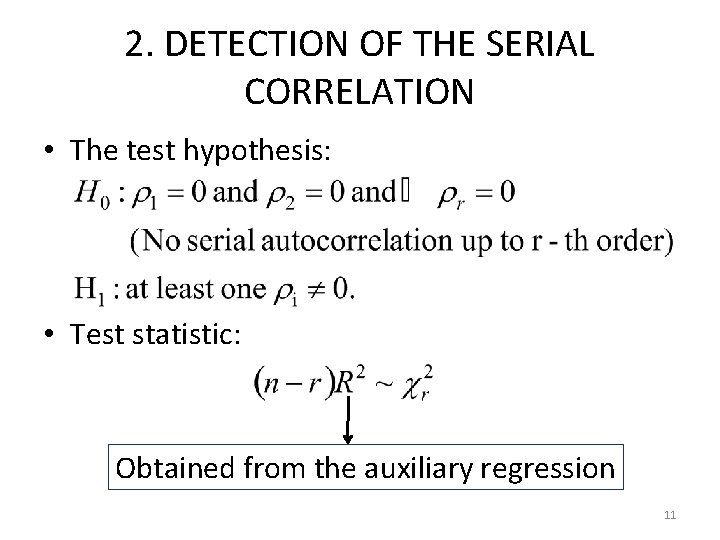
2. DETECTION OF THE SERIAL CORRELATION • The test hypothesis: • Test statistic: Obtained from the auxiliary regression 11

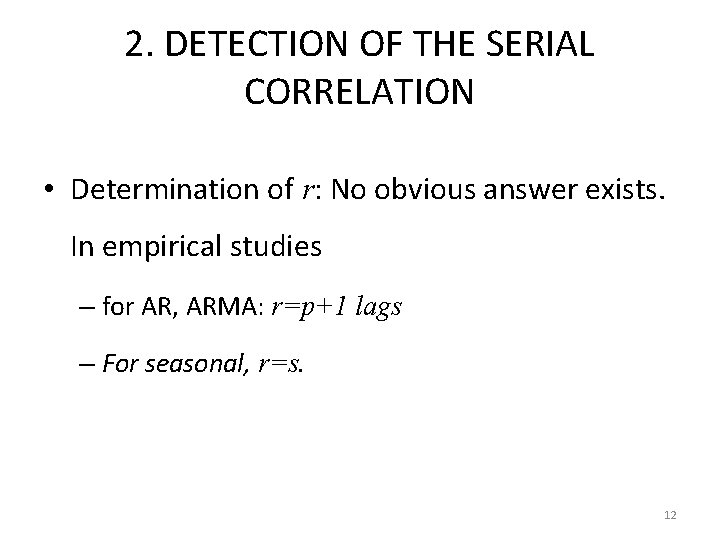
2. DETECTION OF THE SERIAL CORRELATION • Determination of r: No obvious answer exists. In empirical studies – for AR, ARMA: r=p+1 lags – For seasonal, r=s. 12

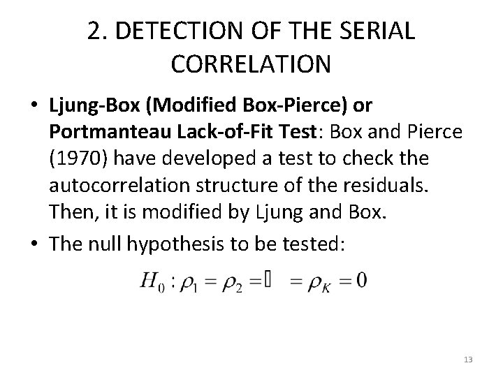
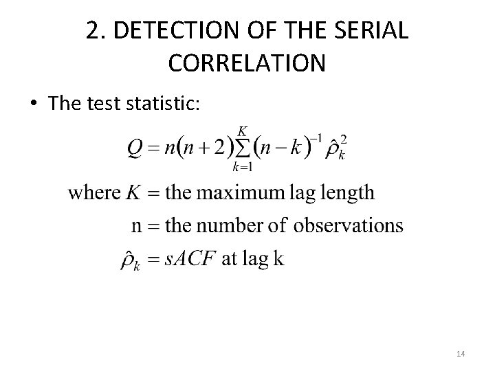
2. DETECTION OF THE SERIAL CORRELATION • Ljung-Box (Modified Box-Pierce) or Portmanteau Lack-of-Fit Test: Box and Pierce (1970) have developed a test to check the autocorrelation structure of the residuals. Then, it is modified by Ljung and Box. • The null hypothesis to be tested: 13

2. DETECTION OF THE SERIAL CORRELATION • The test statistic: 14

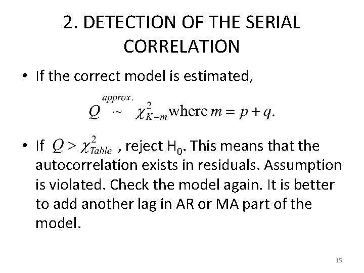
2. DETECTION OF THE SERIAL CORRELATION • If the correct model is estimated, • If , reject H 0. This means that the autocorrelation exists in residuals. Assumption is violated. Check the model again. It is better to add another lag in AR or MA part of the model. 15

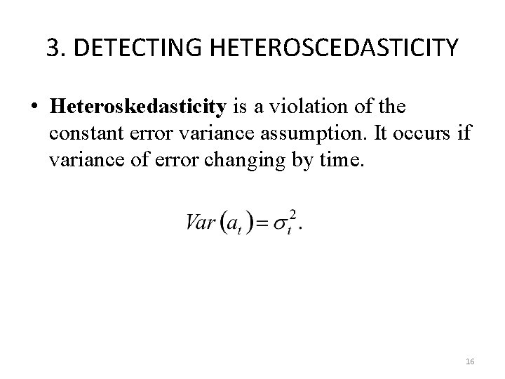
3. DETECTING HETEROSCEDASTICITY • Heteroskedasticity is a violation of the constant error variance assumption. It occurs if variance of error changing by time. 16

3. DETECTING HETEROSCEDASTICITY • ACF-PACF PLOT OF SQUARED RESIDUALS: Since {at} is a zero mean process, the variance of at is defined by the expected value of squared at’s. So, if at’s are homoscedastic, the variance will be constant (not change over time) and when we look at the ACF and PACF plots of squared residuals, they should be in 95% WN limits. If not, this is a sign of heteroscedasticity. 17

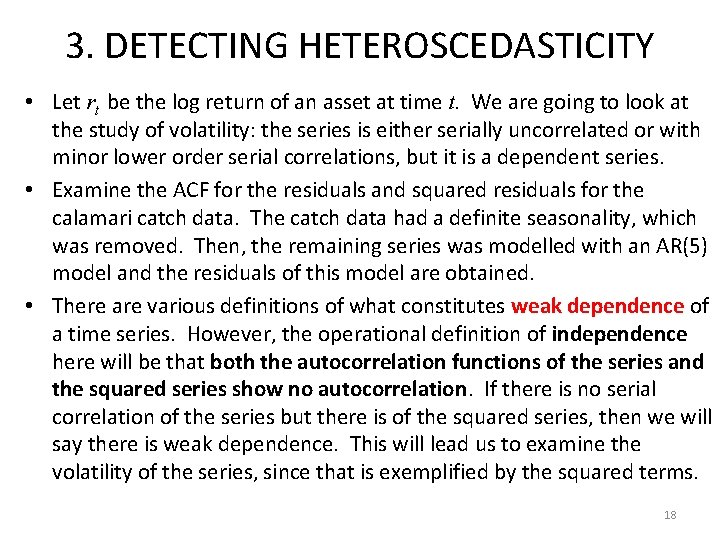
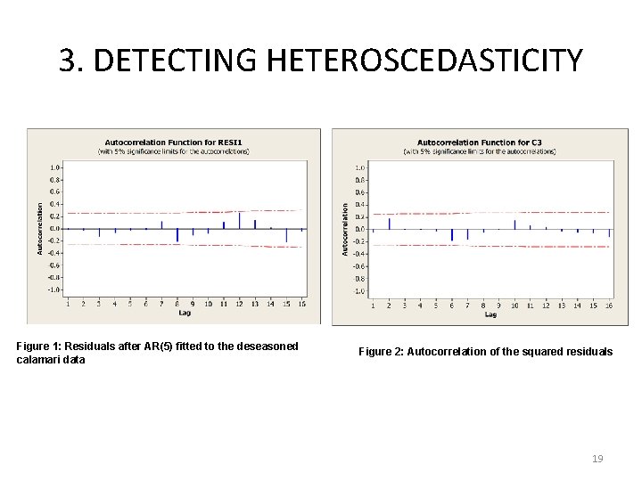
3. DETECTING HETEROSCEDASTICITY • Let rt be the log return of an asset at time t. We are going to look at the study of volatility: the series is either serially uncorrelated or with minor lower order serial correlations, but it is a dependent series. • Examine the ACF for the residuals and squared residuals for the calamari catch data. The catch data had a definite seasonality, which was removed. Then, the remaining series was modelled with an AR(5) model and the residuals of this model are obtained. • There are various definitions of what constitutes weak dependence of a time series. However, the operational definition of independence here will be that both the autocorrelation functions of the series and the squared series show no autocorrelation. If there is no serial correlation of the series but there is of the squared series, then we will say there is weak dependence. This will lead us to examine the volatility of the series, since that is exemplified by the squared terms. 18

3. DETECTING HETEROSCEDASTICITY Figure 1: Residuals after AR(5) fitted to the deseasoned calamari data Figure 2: Autocorrelation of the squared residuals 19

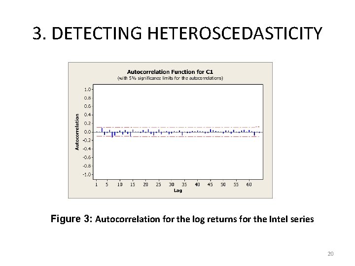
3. DETECTING HETEROSCEDASTICITY Figure 3: Autocorrelation for the log returns for the Intel series 20

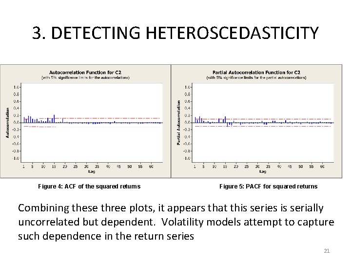
3. DETECTING HETEROSCEDASTICITY Figure 4: ACF of the squared returns Figure 5: PACF for squared returns Combining these three plots, it appears that this series is serially uncorrelated but dependent. Volatility models attempt to capture such dependence in the return series 21

3. DETECTING HETEROSCEDASTICITY • If we ignore heterocedasticity: – The OLS estimator is unbiased but not efficient. The GLS or WLS is the Gauss-Markov estimator. – The estimate of the variance of the OLS estimator is a biased estimator of the true variance. The classical testing procedures are invalidated. • Now, the question is how we can detect heteroscedasticity? 22

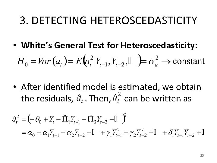
3. DETECTING HETEROSCEDASTICITY • White’s General Test for Heteroscedasticity: • After identified model is estimated, we obtain the residuals, . Then, can be written as 23

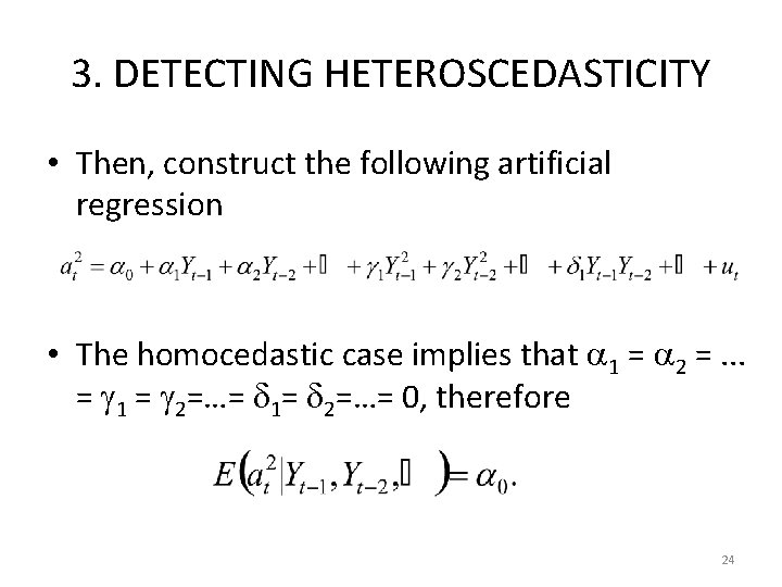
3. DETECTING HETEROSCEDASTICITY • Then, construct the following artificial regression • The homocedastic case implies that 1 = 2 =. . . = 1 = 2=…= 1= 2=…= 0, therefore 24

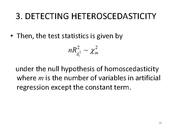
3. DETECTING HETEROSCEDASTICITY • Then, the test statistics is given by under the null hypothesis of homoscedasticity where m is the number of variables in artificial regression except the constant term. 25

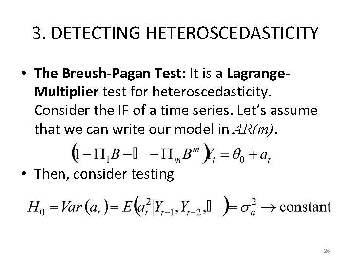
3. DETECTING HETEROSCEDASTICITY • The Breush-Pagan Test: It is a Lagrange. Multiplier test for heteroscedasticity. Consider the IF of a time series. Let’s assume that we can write our model in AR(m). • Then, consider testing 26

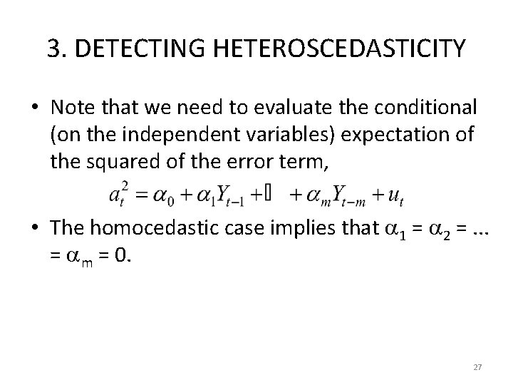
3. DETECTING HETEROSCEDASTICITY • Note that we need to evaluate the conditional (on the independent variables) expectation of the squared of the error term, • The homocedastic case implies that 1 = 2 =. . . = m = 0. 27

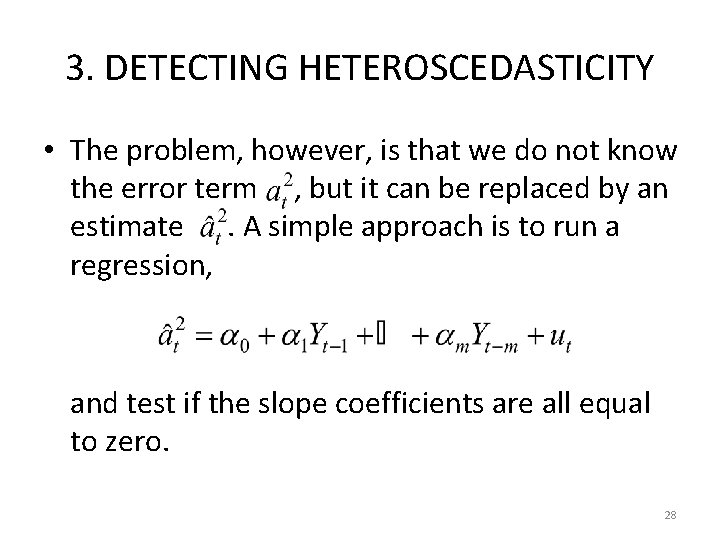
3. DETECTING HETEROSCEDASTICITY • The problem, however, is that we do not know the error term , but it can be replaced by an estimate. A simple approach is to run a regression, and test if the slope coefficients are all equal to zero. 28

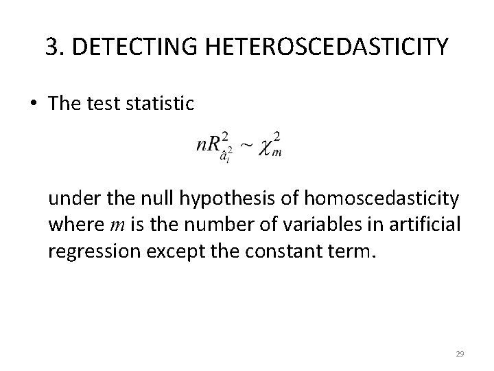
3. DETECTING HETEROSCEDASTICITY • The test statistic under the null hypothesis of homoscedasticity where m is the number of variables in artificial regression except the constant term. 29

3. DETECTING HETEROSCEDASTICITY • If we reject the null hypothesis, this means that the error variance is not constant. It is changing over time. Therefore, we need to model the volatility. ARCH (Autoregressive Conditional Heteroskedasticity) or GARCH (Generalized Autoregressive Conditional Heteroskedasticity) modeling helps us to model the error variance. 30

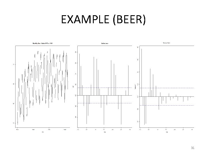
EXAMPLE (BEER) 31

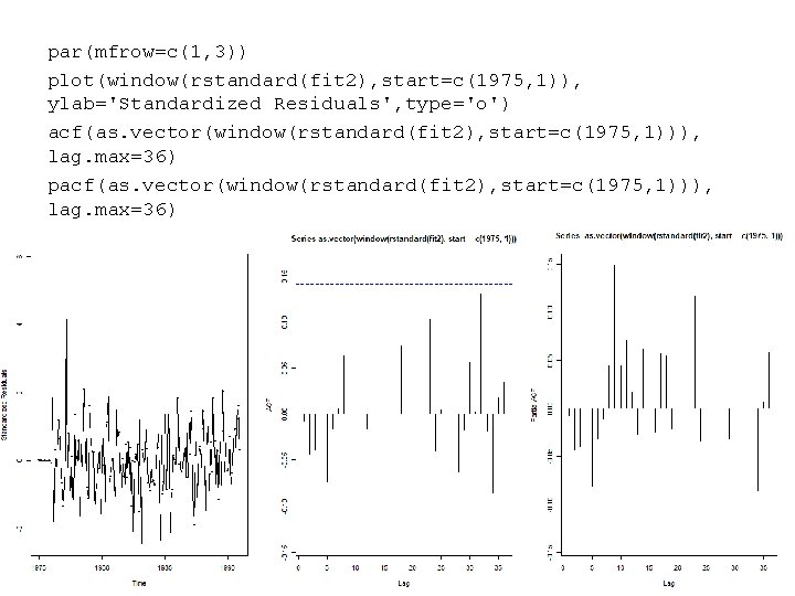
par(mfrow=c(1, 3)) plot(window(rstandard(fit 2), start=c(1975, 1)), ylab='Standardized Residuals', type='o') acf(as. vector(window(rstandard(fit 2), start=c(1975, 1))), lag. max=36) pacf(as. vector(window(rstandard(fit 2), start=c(1975, 1))), lag. max=36) 32

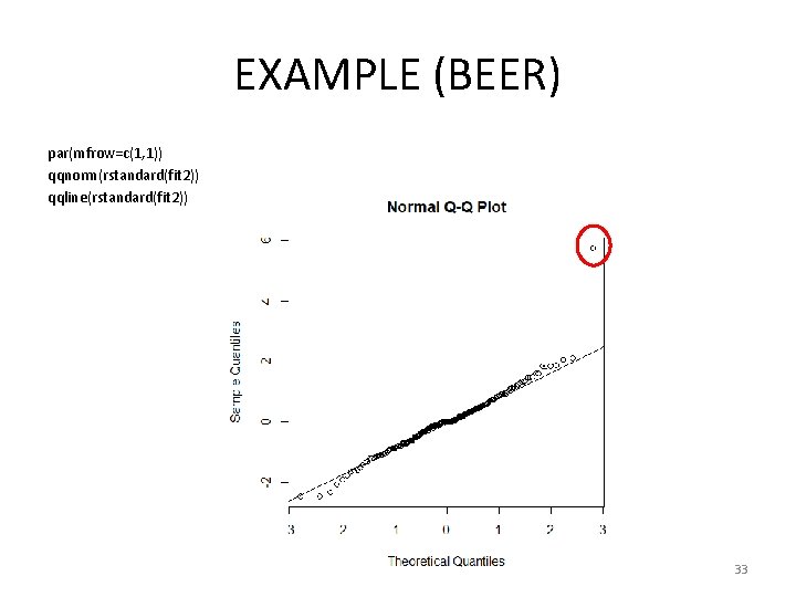
EXAMPLE (BEER) par(mfrow=c(1, 1)) qqnorm(rstandard(fit 2)) qqline(rstandard(fit 2)) 33

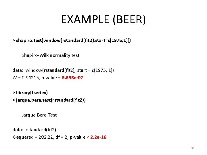
EXAMPLE (BEER) > shapiro. test(window(rstandard(fit 2), start=c(1975, 1))) Shapiro-Wilk normality test data: window(rstandard(fit 2), start = c(1975, 1)) W = 0. 94215, p-value = 5. 658 e-07 > library(tseries) > jarque. bera. test(rstandard(fit 2)) Jarque Bera Test data: rstandard(fit 2) X-squared = 282. 22, df = 2, p-value < 2. 2 e-16 34

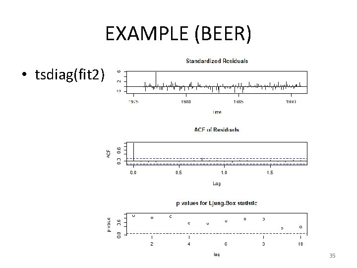
EXAMPLE (BEER) • tsdiag(fit 2) 35

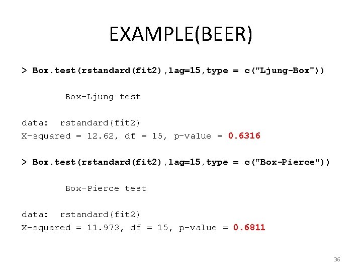
EXAMPLE(BEER) > Box. test(rstandard(fit 2), lag=15, type = c("Ljung-Box")) Box-Ljung test data: rstandard(fit 2) X-squared = 12. 62, df = 15, p-value = 0. 6316 > Box. test(rstandard(fit 2), lag=15, type = c("Box-Pierce")) Box-Pierce test data: rstandard(fit 2) X-squared = 11. 973, df = 15, p-value = 0. 6811 36

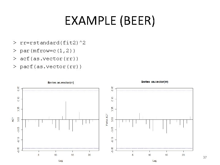
EXAMPLE (BEER) > > rr=rstandard(fit 2)^2 par(mfrow=c(1, 2)) acf(as. vector(rr)) pacf(as. vector(rr)) 37

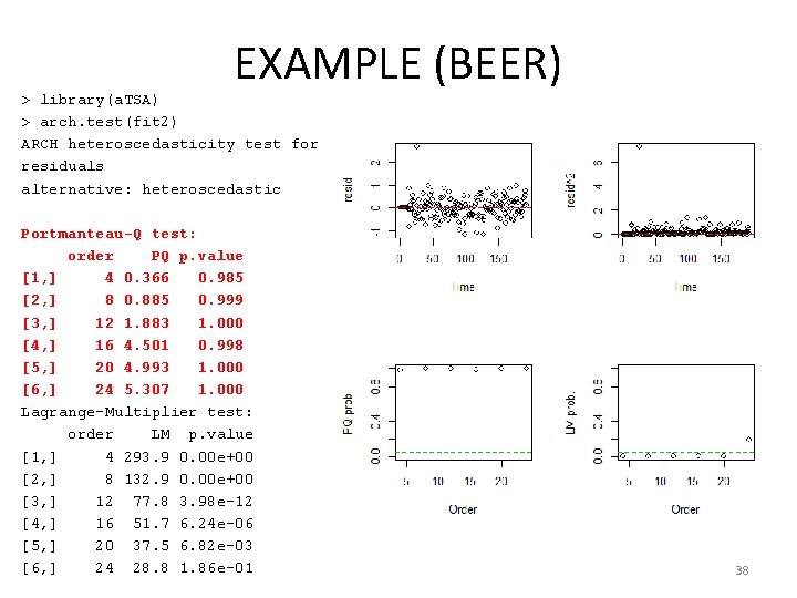
EXAMPLE (BEER) > library(a. TSA) > arch. test(fit 2) ARCH heteroscedasticity test for residuals alternative: heteroscedastic Portmanteau-Q test: order PQ p. value [1, ] 4 0. 366 0. 985 [2, ] 8 0. 885 0. 999 [3, ] 12 1. 883 1. 000 [4, ] 16 4. 501 0. 998 [5, ] 20 4. 993 1. 000 [6, ] 24 5. 307 1. 000 Lagrange-Multiplier test: order LM p. value [1, ] 4 293. 9 0. 00 e+00 [2, ] 8 132. 9 0. 00 e+00 [3, ] 12 77. 8 3. 98 e-12 [4, ] 16 51. 7 6. 24 e-06 [5, ] 20 37. 5 6. 82 e-03 [6, ] 24 28. 8 1. 86 e-01 38

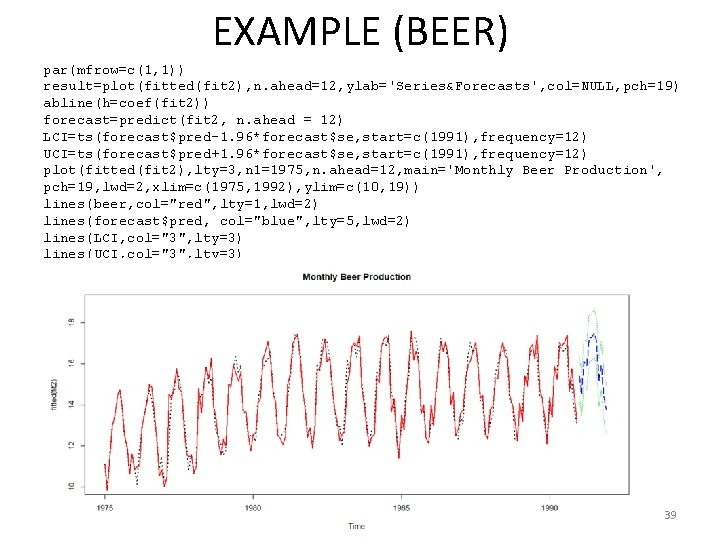
EXAMPLE (BEER) par(mfrow=c(1, 1)) result=plot(fitted(fit 2), n. ahead=12, ylab='Series&Forecasts', col=NULL, pch=19) abline(h=coef(fit 2)) forecast=predict(fit 2, n. ahead = 12) LCI=ts(forecast$pred-1. 96*forecast$se, start=c(1991), frequency=12) UCI=ts(forecast$pred+1. 96*forecast$se, start=c(1991), frequency=12) plot(fitted(fit 2), lty=3, n 1=1975, n. ahead=12, main='Monthly Beer Production', pch=19, lwd=2, xlim=c(1975, 1992), ylim=c(10, 19)) lines(beer, col="red", lty=1, lwd=2) lines(forecast$pred, col="blue", lty=5, lwd=2) lines(LCI, col="3", lty=3) lines(UCI, col="3", lty=3) 39

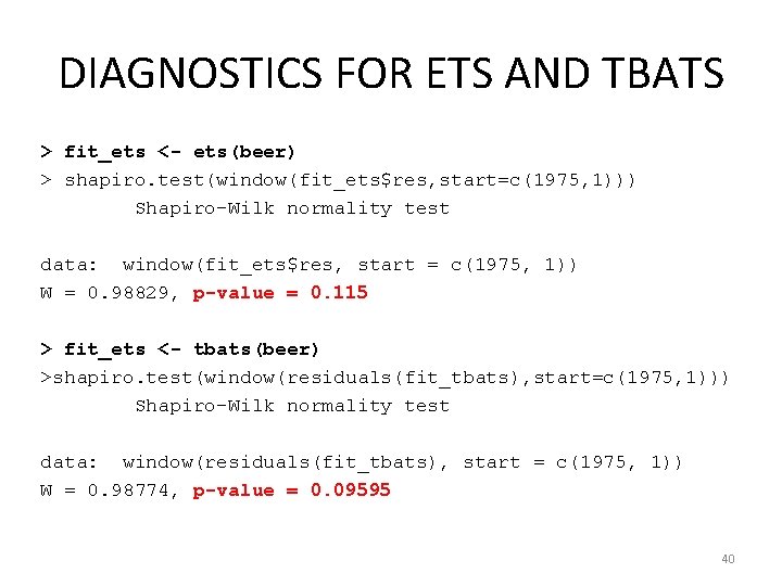
DIAGNOSTICS FOR ETS AND TBATS > fit_ets <- ets(beer) > shapiro. test(window(fit_ets$res, start=c(1975, 1))) Shapiro-Wilk normality test data: window(fit_ets$res, start = c(1975, 1)) W = 0. 98829, p-value = 0. 115 > fit_ets <- tbats(beer) >shapiro. test(window(residuals(fit_tbats), start=c(1975, 1))) Shapiro-Wilk normality test data: window(residuals(fit_tbats), start = c(1975, 1)) W = 0. 98774, p-value = 0. 09595 40