CS 497 Frontiers of Computer Science Introduction to

CS 497 Frontiers of Computer Science Introduction to Quantum Computing Lecture 1 of 2 http: //www. cs. uwaterloo. ca/~cleve/CS 497 -F 07 Richard Cleve David R. Cheriton School of Computer Science Institute for Quantum Computing University of Waterloo October 1 & 3, 2007 1

Contents of lecture 1 1. 2. 3. 4. 5. 6. 7. Preliminary remarks Quantum states Unitary operations & measurements Subsystem structure & quantum circuit diagrams Introductory remarks about quantum algorithms Deutsch’s parity algorithm One-out-of-four search algorithm 2

Contents of lecture 1 1. 2. 3. 4. 5. 6. 7. Preliminary remarks Quantum states Unitary operations & measurements Subsystem structure & quantum circuit diagrams Introductory remarks about quantum algorithms Deutsch’s parity algorithm One-out-of-four search algorithm 3

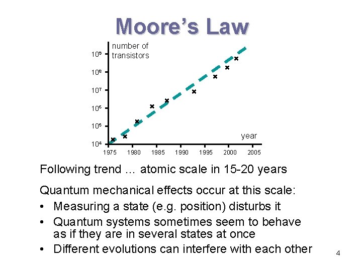
Moore’s Law 109 number of transistors 108 107 106 105 year 104 1975 1980 1985 1990 1995 2000 2005 Following trend … atomic scale in 15 -20 years Quantum mechanical effects occur at this scale: • Measuring a state (e. g. position) disturbs it • Quantum systems sometimes seem to behave as if they are in several states at once • Different evolutions can interfere with each other 4

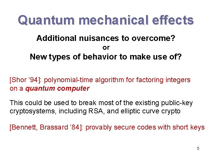
Quantum mechanical effects Additional nuisances to overcome? or New types of behavior to make use of? [Shor ’ 94]: polynomial-time algorithm for factoring integers on a quantum computer This could be used to break most of the existing public-key cryptosystems, including RSA, and elliptic curve crypto [Bennett, Brassard ’ 84]: provably secure codes with short keys 5

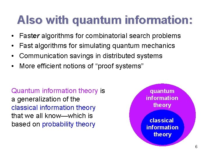
Also with quantum information: • • Faster algorithms for combinatorial search problems Fast algorithms for simulating quantum mechanics Communication savings in distributed systems More efficient notions of “proof systems” Quantum information theory is a generalization of the classical information theory that we all know—which is based on probability theory quantum information theory classical information theory 6

Contents of lecture 1 1. 2. 3. 4. 5. 6. 7. Preliminary remarks Quantum states Unitary operations & measurements Subsystem structure & quantum circuit diagrams Introductory remarks about quantum algorithms Deutsch’s parity algorithm One-out-of-four search algorithm 7

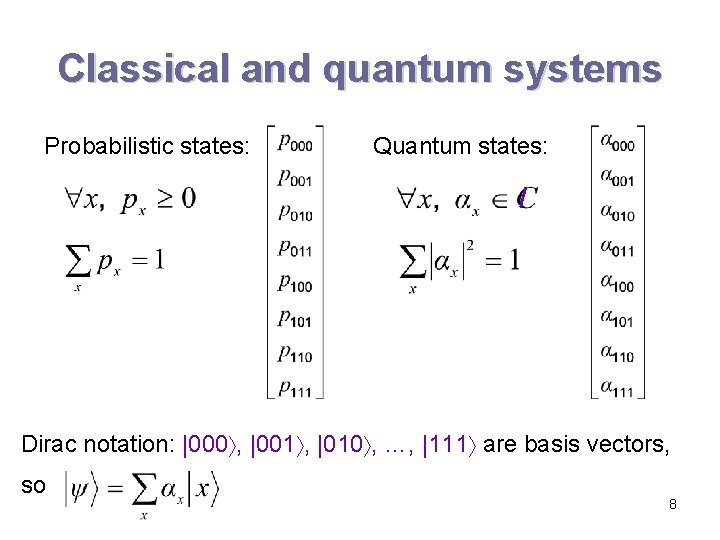
Classical and quantum systems Probabilistic states: Quantum states: Dirac notation: |000 , |001 , |010 , …, |111 are basis vectors, so 8

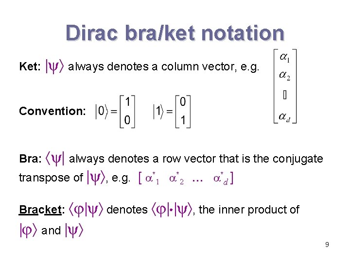
Dirac bra/ket notation Ket: ψ always denotes a column vector, e. g. Convention: Bra: ψ always denotes a row vector that is the conjugate transpose of ψ , e. g. [ *1 *2 *d ] Bracket: φ ψ denotes φ ψ , the inner product of φ and ψ 9

Contents of lecture 1 1. 2. 3. 4. 5. 6. 7. Preliminary remarks Quantum states Unitary operations & measurements Subsystem structure & quantum circuit diagrams Introductory remarks about quantum algorithms Deutsch’s parity algorithm One-out-of-four search algorithm 10

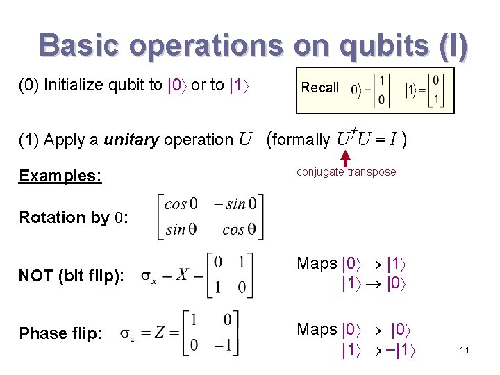
Basic operations on qubits (I) (0) Initialize qubit to |0 or to |1 Recall † (1) Apply a unitary operation U (formally U U = I ) Examples: conjugate transpose Rotation by : NOT (bit flip): Maps |0 |1 |1 |0 Phase flip: Maps |0 |1 |1 11

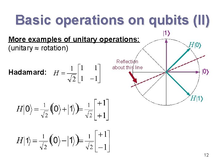
Basic operations on qubits (II) More examples of unitary operations: (unitary rotation) Hadamard: Reflection about this line 1 H 0 0 H 1 12

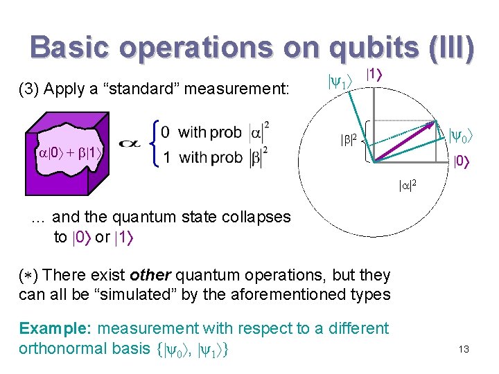
Basic operations on qubits (III) (3) Apply a “standard” measurement: 0 + 1 ψ1 1 ψ0 | |2 0 | |2 … and the quantum state collapses to 0 or 1 ( ) There exist other quantum operations, but they can all be “simulated” by the aforementioned types Example: measurement with respect to a different orthonormal basis { ψ0 , ψ1 } 13

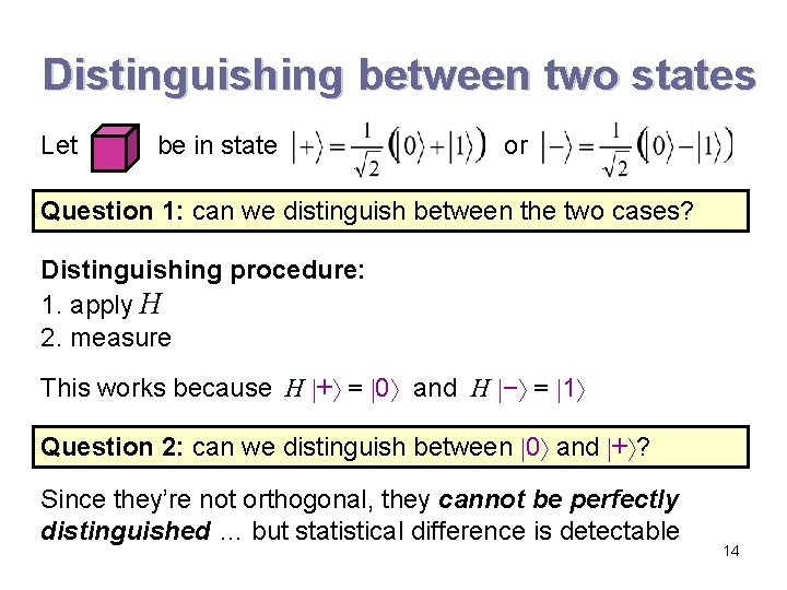
Distinguishing between two states Let be in state or Question 1: can we distinguish between the two cases? Distinguishing procedure: 1. apply H 2. measure This works because H + = 0 and H − = 1 Question 2: can we distinguish between 0 and + ? Since they’re not orthogonal, they cannot be perfectly distinguished … but statistical difference is detectable 14

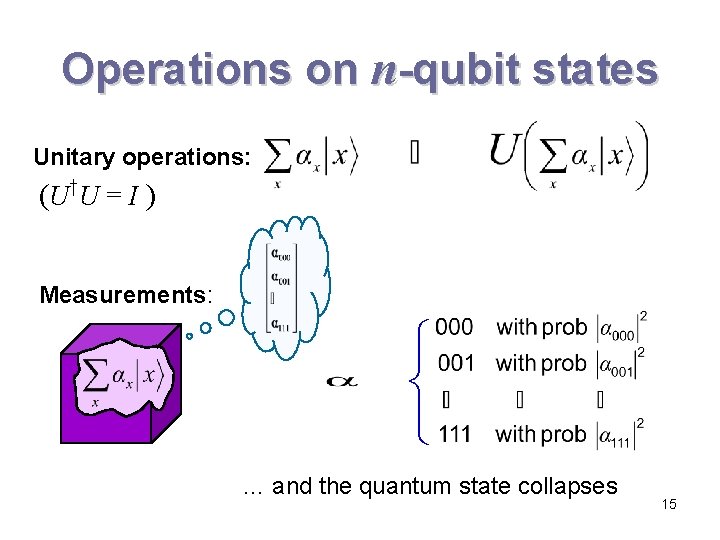
Operations on n-qubit states Unitary operations: ( U †U = I ) Measurements: … and the quantum state collapses 15

Contents of lecture 1 1. 2. 3. 4. 5. 6. 7. Preliminary remarks Quantum states Unitary operations & measurements Subsystem structure & quantum circuit diagrams Introductory remarks about quantum algorithms Deutsch’s parity algorithm One-out-of-four search algorithm 16

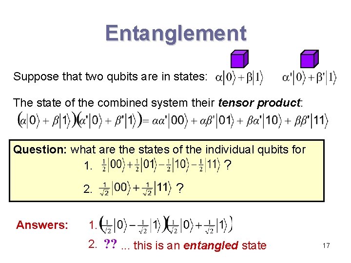
Entanglement Suppose that two qubits are in states: The state of the combined system their tensor product: Question: what are the states of the individual qubits for 1. ? 2. Answers: ? 1. 2. ? ? . . . this is an entangled state 17

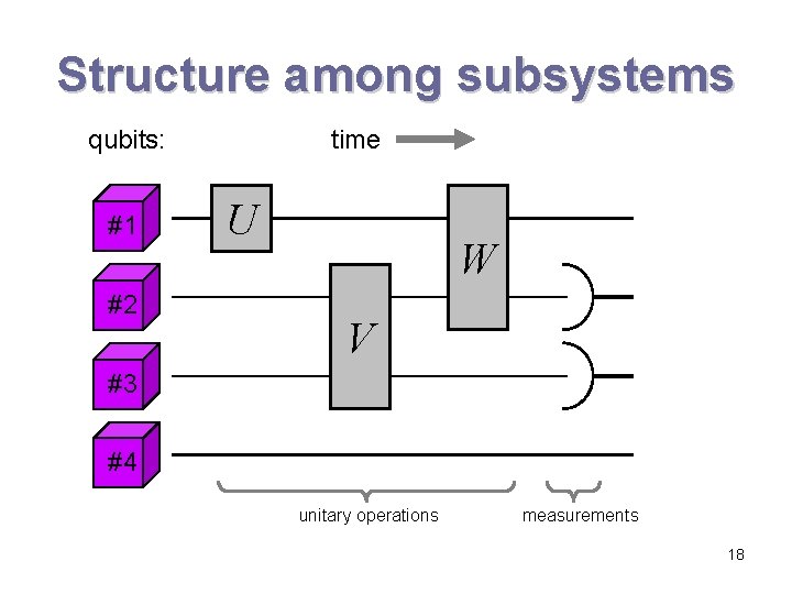
Structure among subsystems qubits: #1 #2 time U W V #3 #4 unitary operations measurements 18

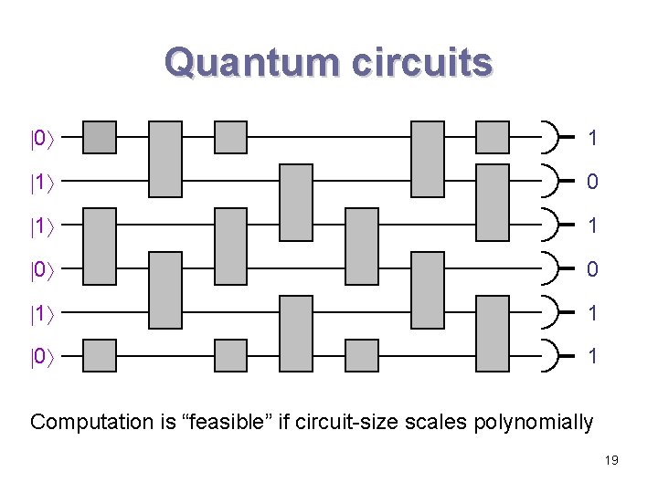
Quantum circuits 0 1 1 0 1 Computation is “feasible” if circuit-size scales polynomially 19

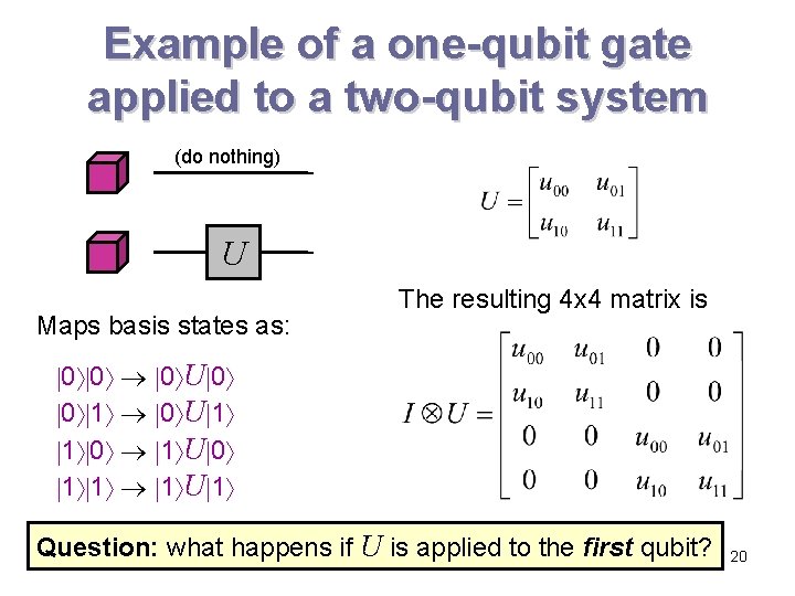
Example of a one-qubit gate applied to a two-qubit system (do nothing) U Maps basis states as: The resulting 4 x 4 matrix is 0 0 0 U 0 0 1 0 U 1 1 0 1 U 0 1 1 1 U 1 Question: what happens if U is applied to the first qubit? 20

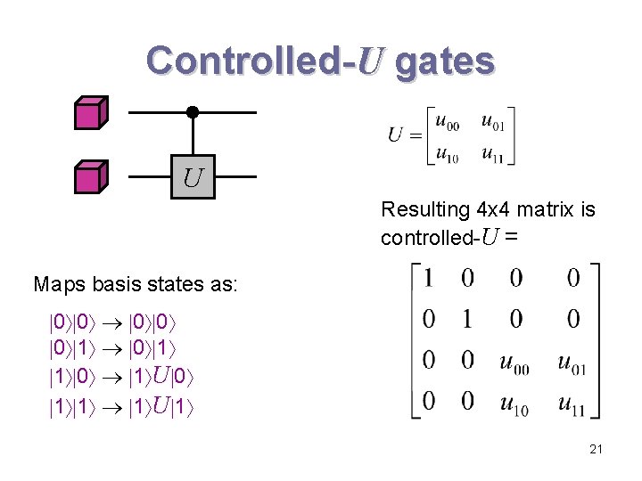
Controlled-U gates U Resulting 4 x 4 matrix is controlled-U = Maps basis states as: 0 0 0 1 1 0 1 U 0 1 1 1 U 1 21

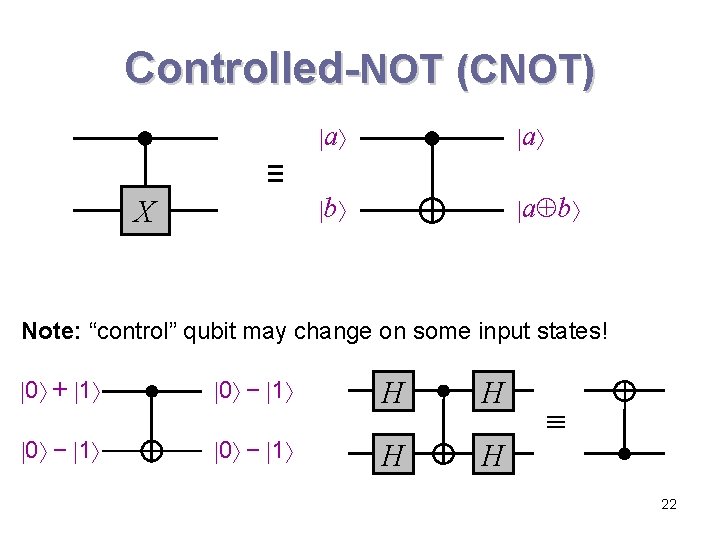
Controlled-NOT (CNOT) a a b a b ≡ X Note: “control” qubit may change on some input states! 0 + 1 0 − 1 H H 22

Contents of lecture 1 1. 2. 3. 4. 5. 6. 7. Preliminary remarks Quantum states Unitary operations & measurements Subsystem structure & quantum circuit diagrams Introductory remarks about quantum algorithms Deutsch’s parity algorithm One-out-of-four search algorithm 23

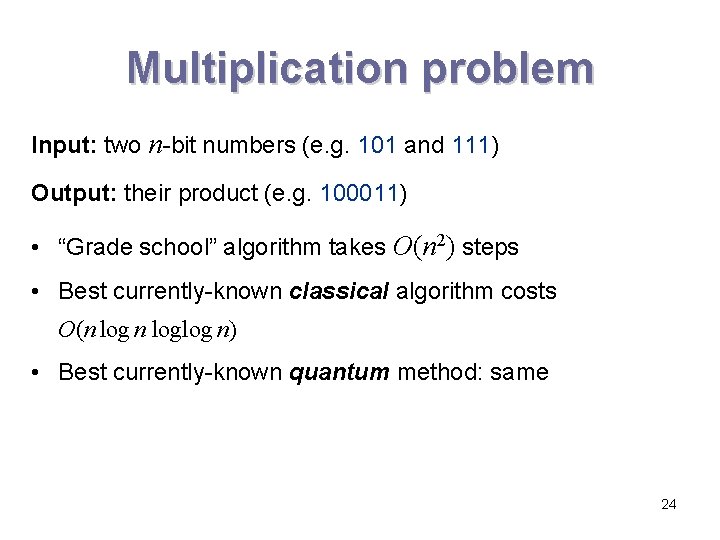
Multiplication problem Input: two n-bit numbers (e. g. 101 and 111) Output: their product (e. g. 100011) • “Grade school” algorithm takes O(n 2) steps • Best currently-known classical algorithm costs O(n loglog n) • Best currently-known quantum method: same 24

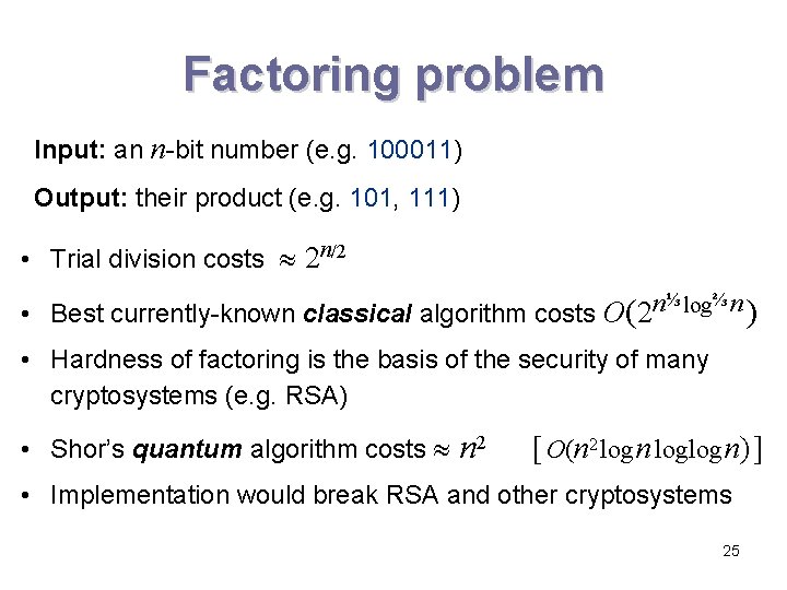
Factoring problem Input: an n-bit number (e. g. 100011) Output: their product (e. g. 101, 111) • Trial division costs 2 n/2 ⅓ ⅔ • Best currently-known classical algorithm costs O(2 n log n ) • Hardness of factoring is the basis of the security of many cryptosystems (e. g. RSA) • Shor’s quantum algorithm costs n 2 [ O(n 2 log n loglog n) ] • Implementation would break RSA and other cryptosystems 25

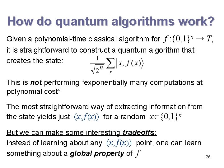
How do quantum algorithms work? Given a polynomial-time classical algorithm for f : {0, 1}n → T, it is straightforward to construct a quantum algorithm that creates the state: This is not performing “exponentially many computations at polynomial cost” The most straightforward way of extracting information from the state yields just (x, f (x)) for a random x {0, 1}n But we can make some interesting tradeoffs: instead of learning about any (x, f (x)) point, one can learn something about a global property of f 26

Contents of lecture 1 1. 2. 3. 4. 5. 6. 7. Preliminary remarks Quantum states Unitary operations & measurements Subsystem structure & quantum circuit diagrams Introductory remarks about quantum algorithms Deutsch’s parity algorithm One-out-of-four search algorithm 27

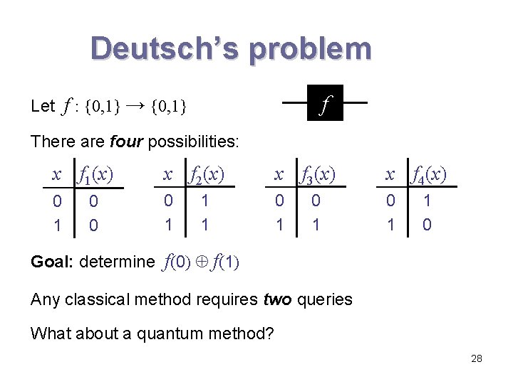
Deutsch’s problem f Let f : {0, 1} → {0, 1} There are four possibilities: x f 1(x) x f 2(x) x f 3(x) x f 4(x) 0 1 0 1 0 0 1 1 0 Goal: determine f(0) f(1) Any classical method requires two queries What about a quantum method? 28

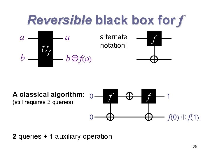
Reversible black box for f a b a Uf alternate notation: f b f(a) A classical algorithm: 0 (still requires 2 queries) f 0 f 1 f(0) f(1) 2 queries + 1 auxiliary operation 29

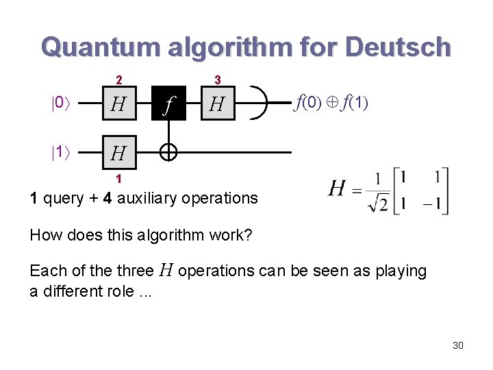
Quantum algorithm for Deutsch 2 0 H 1 H 3 f H f(0) f(1) 1 1 query + 4 auxiliary operations How does this algorithm work? Each of the three H operations can be seen as playing a different role. . . 30

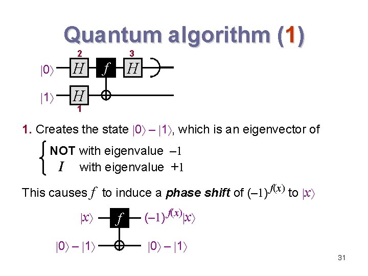
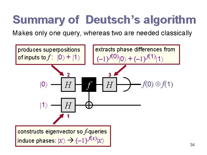
Quantum algorithm (1) 2 0 H 1 H 3 H f 1 1. Creates the state 0 – 1 , which is an eigenvector of NOT with eigenvalue – 1 I with eigenvalue +1 This causes f to induce a phase shift of (– 1) f(x) to x x 0 – 1 f (– 1) f(x) x 0 – 1 31

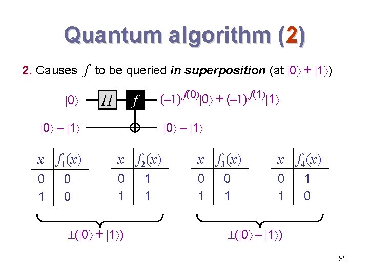
Quantum algorithm (2) 2. Causes f to be queried in superposition (at 0 + 1 ) 0 H (– 1) f(0) 0 + (– 1) f(1) 1 f 0 – 1 x f 1(x) x f 2(x) x f 3(x) x f 4(x) 0 1 0 1 0 0 ( 0 + 1 ) 1 1 0 ( 0 – 1 ) 32

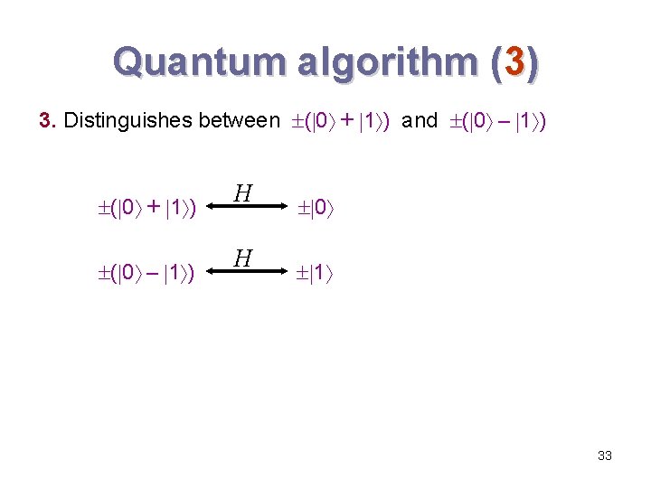
Quantum algorithm (3) 3. Distinguishes between ( 0 + 1 ) and ( 0 – 1 ) ( 0 + 1 ) ( 0 – 1 ) H H 0 1 33

Summary of Deutsch’s algorithm Makes only one query, whereas two are needed classically extracts phase differences from produces superpositions of inputs to f : 0 + 1 (– 1) f(0) 0 + (– 1) f(1) 1 2 0 H 1 H 3 f H f(0) f(1) 1 constructs eigenvector so f-queries induce phases: x (– 1) f(x) x 34

Contents of lecture 1 1. 2. 3. 4. 5. 6. 7. Preliminary remarks Quantum states Unitary operations & measurements Subsystem structure & quantum circuit diagrams Introductory remarks about quantum algorithms Deutsch’s parity algorithm One-out-of-four search algorithm 35

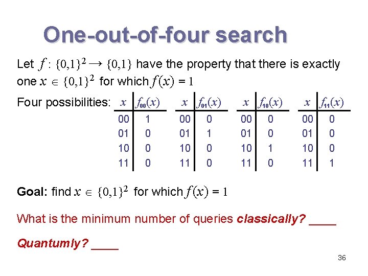
One-out-of-four search Let f : {0, 1}2 → {0, 1} have the property that there is exactly one x {0, 1}2 for which f (x) = 1 Four possibilities: x f 00(x) 00 01 10 11 1 0 0 0 x f 01(x) x f 10(x) x f 11(x) 00 01 10 11 0 0 0 0 1 Goal: find x {0, 1}2 for which f (x) = 1 What is the minimum number of queries classically? ____ Quantumly? ____ 36

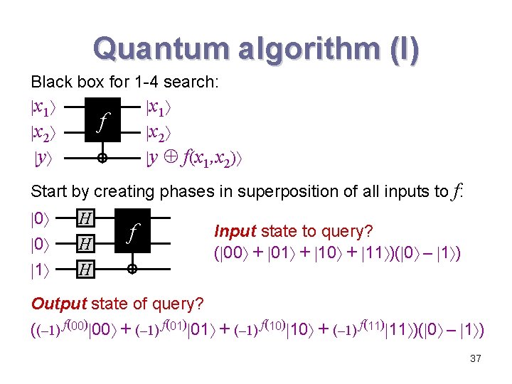
Quantum algorithm (I) Black box for 1 -4 search: x 1 f x 2 y y f(x 1, x 2) Start by creating phases in superposition of all inputs to f: 0 0 1 H H H f Input state to query? ( 00 + 01 + 10 + 11 )( 0 – 1 ) Output state of query? ((– 1) f(00) 00 + (– 1) f(01) 01 + (– 1) f(10) 10 + (– 1) f(11) 11 )( 0 – 1 ) 37

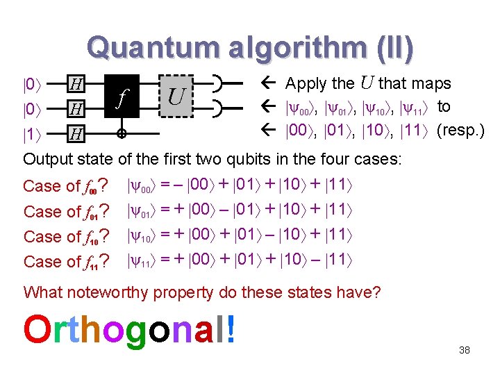
Quantum algorithm (II) 0 H f U Apply the U that maps ψ00 , ψ01 , ψ10 , ψ11 to 00 , 01 , 10 , 11 (resp. ) H 0 H 1 Output state of the first two qubits in the four cases: Case of f 00? ψ00 = – 00 + 01 + 10 + 11 Case of f 01? ψ01 = + 00 – 01 + 10 + 11 Case of f 10? ψ10 = + 00 + 01 – 10 + 11 Case of f 11? ψ11 = + 00 + 01 + 10 – 11 What noteworthy property do these states have? Orthogonal! 38

39