STAT 497 APPLIED TIME SERIES ANALYSIS INTRODUCTION 1

STAT 497 APPLIED TIME SERIES ANALYSIS INTRODUCTION 1

TIME SERIES • Whether we wish to predict the trend in financial markets or electricity consumption, time is an important factor that must be considered in our models. • A time series is simply a series of data points ordered in time. In a time series, time is often the independent variable and the goal is usually to make a forecast for the future. 2

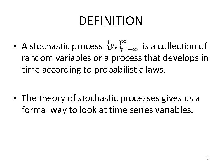
DEFINITION • A stochastic process is a collection of random variables or a process that develops in time according to probabilistic laws. • The theory of stochastic processes gives us a formal way to look at time series variables. 3

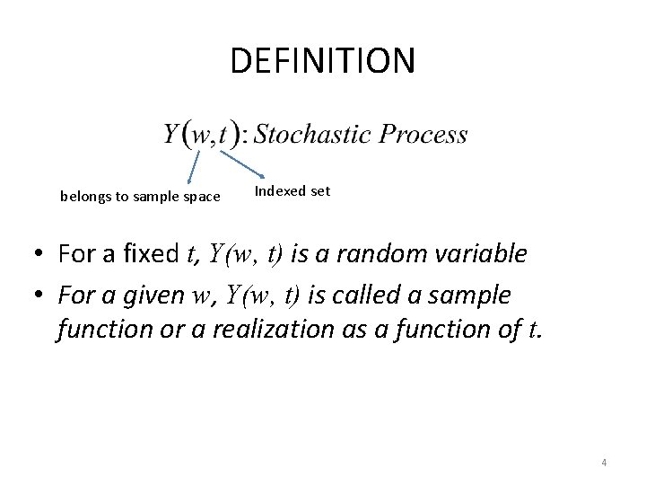
DEFINITION belongs to sample space Indexed set • For a fixed t, Y(w, t) is a random variable • For a given w, Y(w, t) is called a sample function or a realization as a function of t. 4

DEFINITION • Time series is a realization or sample function from a certain stochastic process. • A time series is a set of observations generated sequentially in time. Therefore, they are dependent to each other. This means that we do NOT have a random sample. • We assume that observations are equally spaced in time. • We also assume that closer observations might have stronger dependency. 5

• Let us understand this with an example. Let’s say India expanded its military strength of 1. 5 active military personals in 2018 to 2 million in 2019. That is, of course, an increase in power, sure increase in military strength is not all to determine power but let’s suppose it is. We know that in just one-year India strengthened its military with half a million soldiers. • A closer look shows how much Indian military has strengthened in a year. Clearly, we can see something is dependent on time. And say we have reasonable records proving the change in the number over different points of time and then we call it dataset and we can use it to predict the number for future. Now, this is Time Series Analysis. • We cannot predict the result of a war with the number of soldiers but we sure can predict the number of soldiers with the data. And that is the power of data. 6

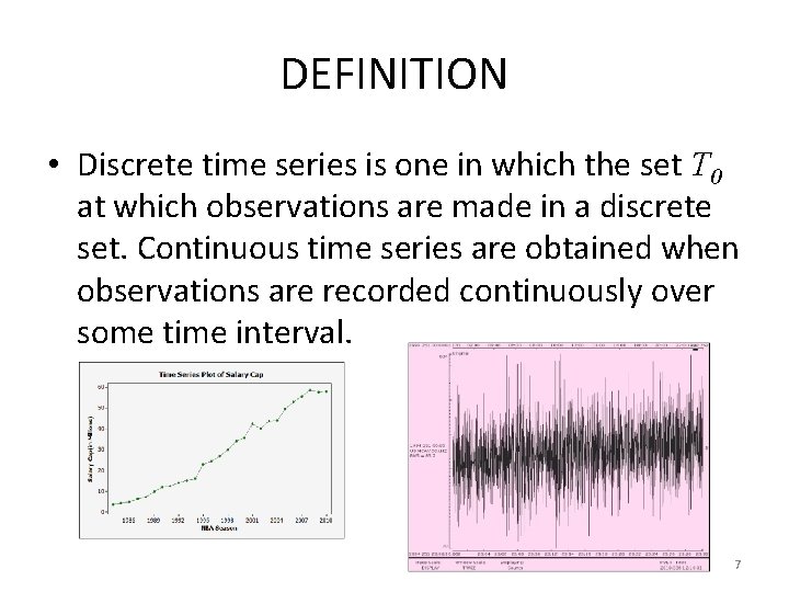
DEFINITION • Discrete time series is one in which the set T 0 at which observations are made in a discrete set. Continuous time series are obtained when observations are recorded continuously over some time interval. 7

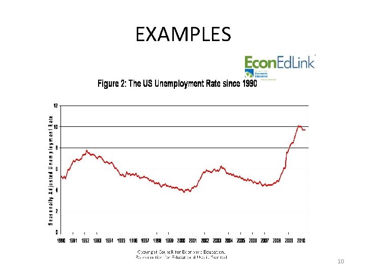
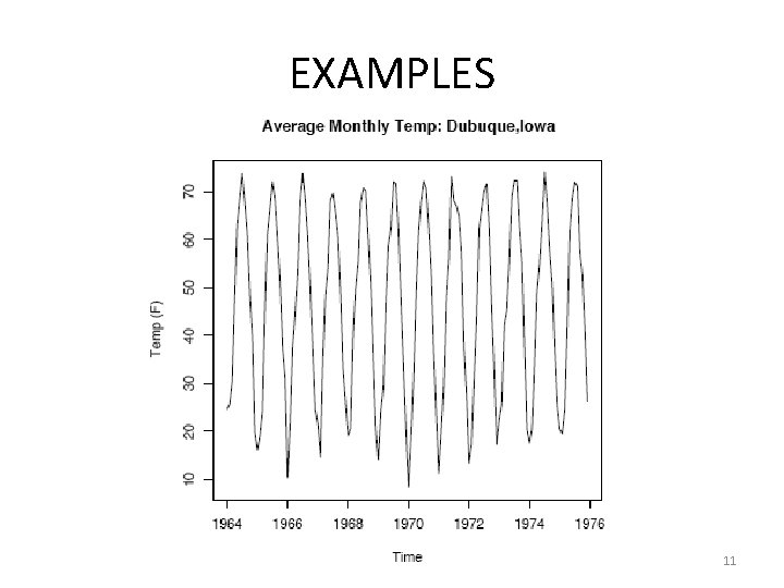
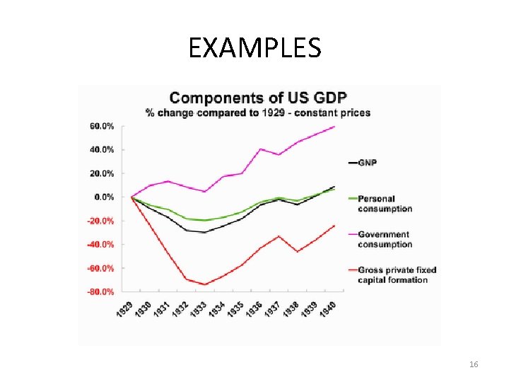
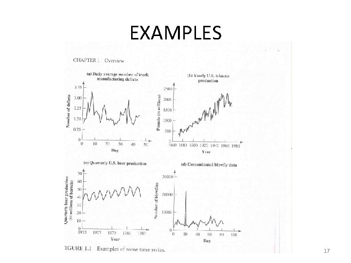
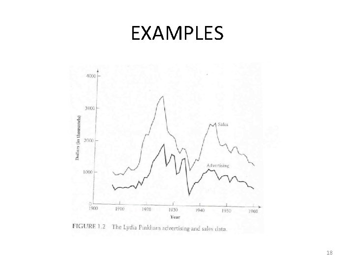
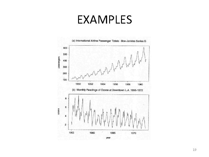
EXAMPLES • Data in business, economics, engineering, environment, medicine, earth sciences, and other areas of scientific investigations are often collected in the form of time series. • Hourly temperature readings • Daily stock prices • Weekly traffic volume • Annual growth rate • Seasonal ice cream consumption • Electrical signals 8

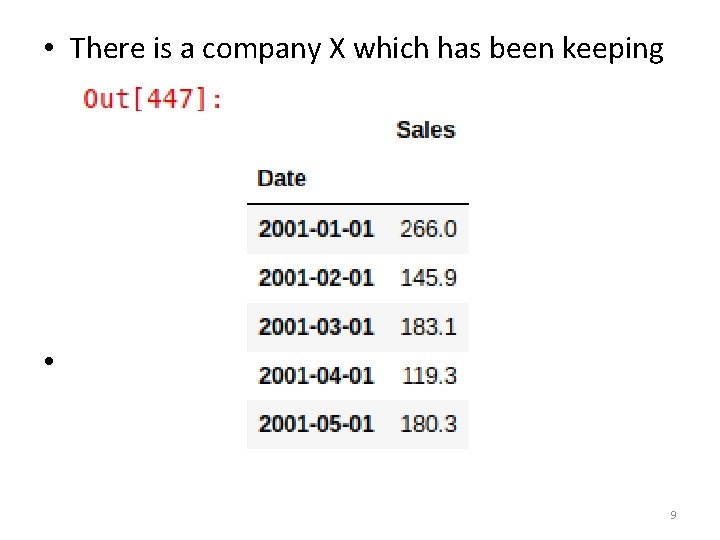
• There is a company X which has been keeping a record of monthly sales of shampoo for the past 3 years. Company X wants to forecast the sale of the shampoo for the next 4 months so that the demand supply gap can be managed by the organization. Our main job here is to simply predict the sales of the shampoo for the next 4 months. • Dataset comprises of only two columns. One is the Date of the month and other is the sale of the shampoo in that month. 9

EXAMPLES 10

EXAMPLES 11

EXAMPLES 12

EXAMPLES 13

EXAMPLES 14

EXAMPLES 15

EXAMPLES 16

EXAMPLES 17

EXAMPLES 18

EXAMPLES 19

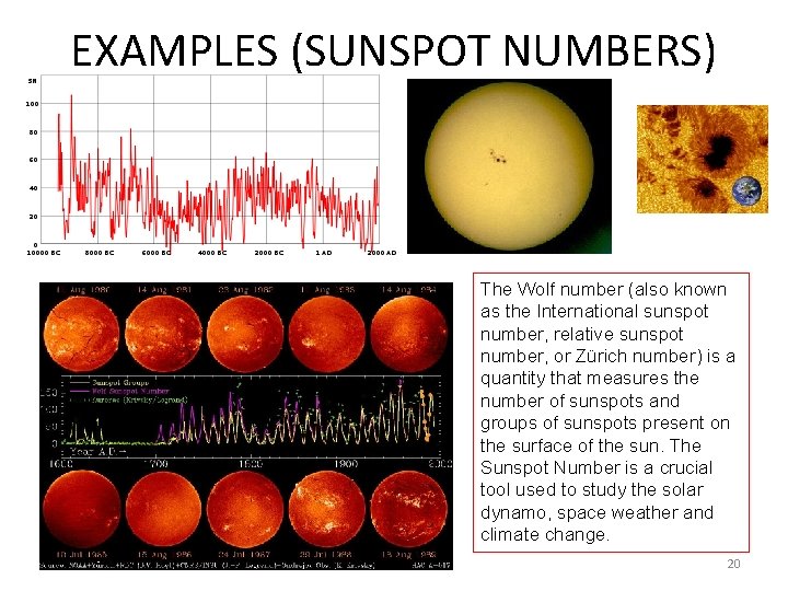
EXAMPLES (SUNSPOT NUMBERS) The Wolf number (also known as the International sunspot number, relative sunspot number, or Zürich number) is a quantity that measures the number of sunspots and groups of sunspots present on the surface of the sun. The Sunspot Number is a crucial tool used to study the solar dynamo, space weather and climate change. 20

OBJECTIVES OF TIME SERIES ANALYSIS • Understanding the dynamic or timedependent structure of the observations of a single series (univariate analysis) • Forecasting of future observations • Ascertaining the leading, lagging and feedback relationships among several series (multivariate analysis) 21

STEPS IN TIME SERIES ANALYSIS • Model Identification – – Time Series plot of the series Check for the existence of a trend or seasonality Check for the sharp changes in behavior Check for possible outliers • Remove the trend and the seasonal component to get stationary residuals. • Estimation – MME – MLE • Diagnostic Checking – Normality of error terms – Independency of error terms – Constant error variance (Homoscedasticity) • Forecasting – Exponential smoothing methods – Minimum MSE forecasting 22

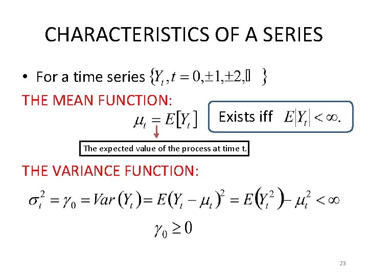
CHARACTERISTICS OF A SERIES • For a time series THE MEAN FUNCTION: Exists iff The expected value of the process at time t. THE VARIANCE FUNCTION: 23

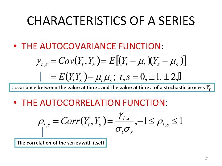
CHARACTERISTICS OF A SERIES • THE AUTOCOVARIANCE FUNCTION: Covariance between the value at time t and the value at time s of a stochastic process Yt. • THE AUTOCORRELATION FUNCTION: The correlation of the series with itself 24

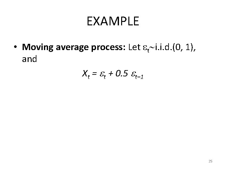
EXAMPLE • Moving average process: Let t i. i. d. (0, 1), and Xt = t + 0. 5 t− 1 25

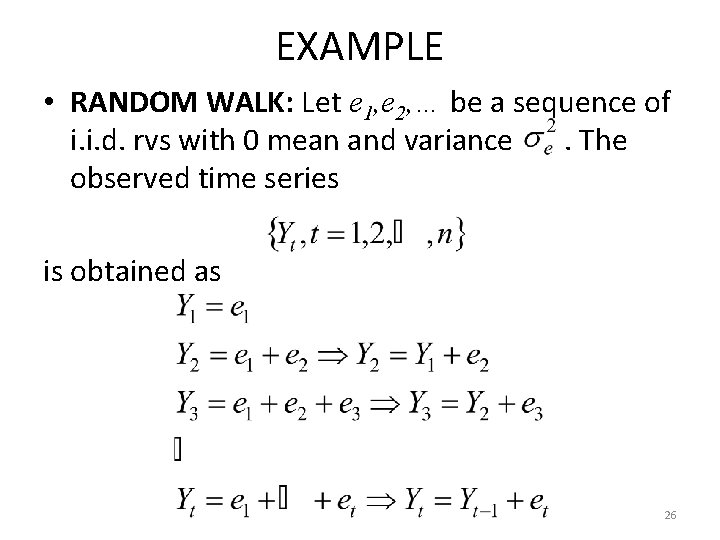
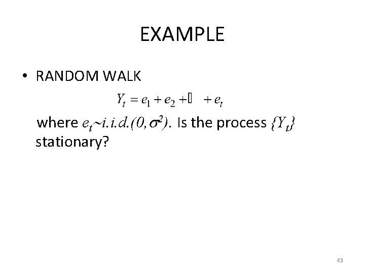
EXAMPLE • RANDOM WALK: Let e 1, e 2, … be a sequence of i. i. d. rvs with 0 mean and variance . The observed time series is obtained as 26

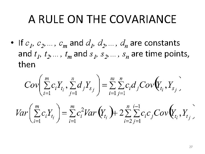
A RULE ON THE COVARIANCE • If c 1, c 2, …, cm and d 1, d 2, …, dn are constants and t 1, t 2, …, tm and s 1, s 2, …, sn are time points, then 27

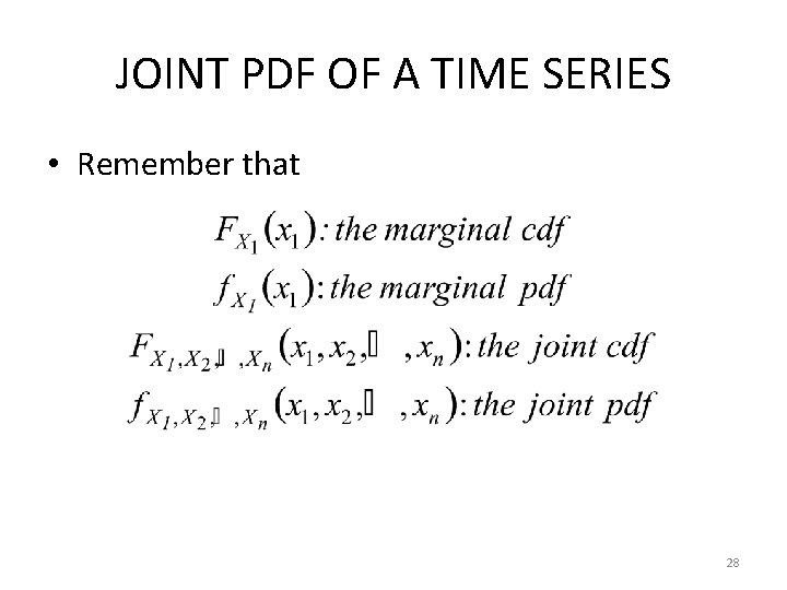
JOINT PDF OF A TIME SERIES • Remember that 28

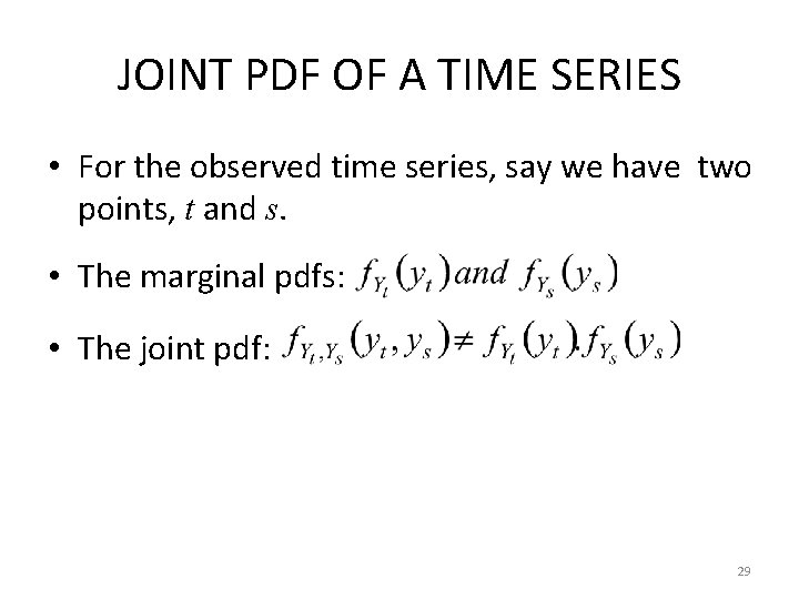
JOINT PDF OF A TIME SERIES • For the observed time series, say we have two points, t and s. • The marginal pdfs: • The joint pdf: 29

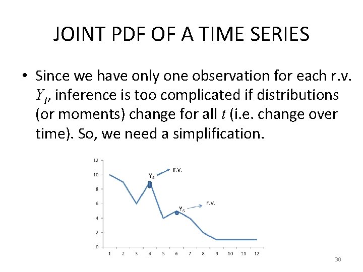
JOINT PDF OF A TIME SERIES • Since we have only one observation for each r. v. Yt, inference is too complicated if distributions (or moments) change for all t (i. e. change over time). So, we need a simplification. r. v. 30

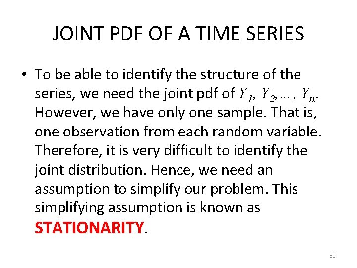
JOINT PDF OF A TIME SERIES • To be able to identify the structure of the series, we need the joint pdf of Y 1, Y 2, …, Yn. However, we have only one sample. That is, one observation from each random variable. Therefore, it is very difficult to identify the joint distribution. Hence, we need an assumption to simplify our problem. This simplifying assumption is known as STATIONARITY. 31

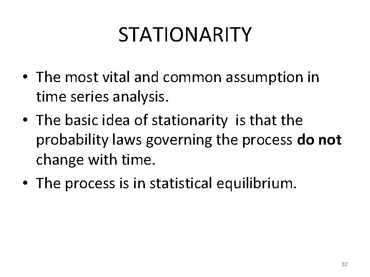
STATIONARITY • The most vital and common assumption in time series analysis. • The basic idea of stationarity is that the probability laws governing the process do not change with time. • The process is in statistical equilibrium. 32

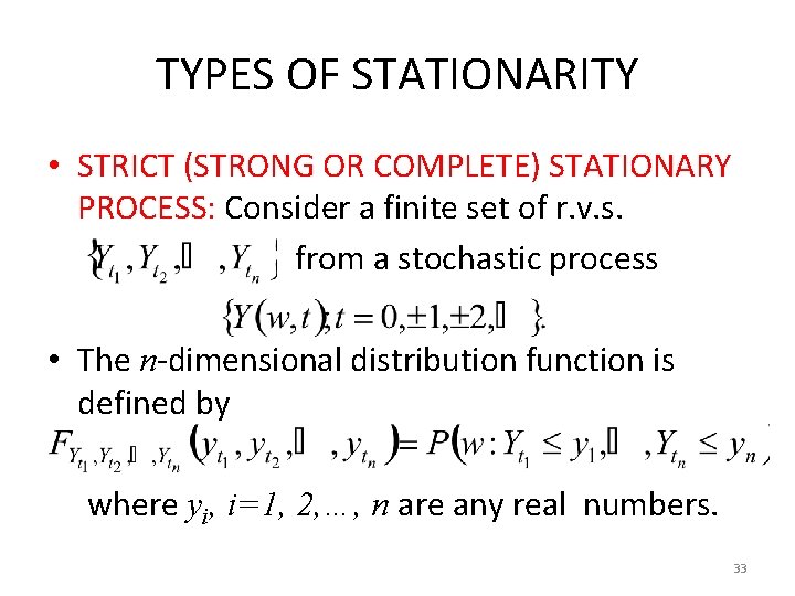
TYPES OF STATIONARITY • STRICT (STRONG OR COMPLETE) STATIONARY PROCESS: Consider a finite set of r. v. s. from a stochastic process • The n-dimensional distribution function is defined by where yi, i=1, 2, …, n are any real numbers. 33

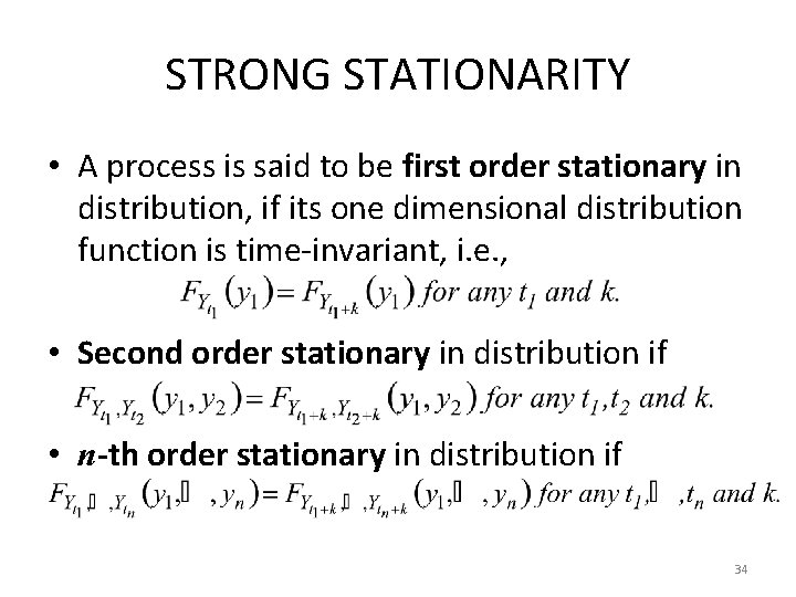
STRONG STATIONARITY • A process is said to be first order stationary in distribution, if its one dimensional distribution function is time-invariant, i. e. , • Second order stationary in distribution if • n-th order stationary in distribution if 34

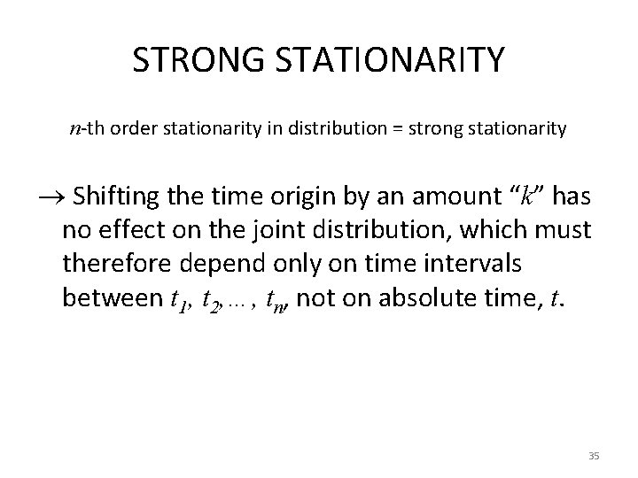
STRONG STATIONARITY n-th order stationarity in distribution = strong stationarity Shifting the time origin by an amount “k” has no effect on the joint distribution, which must therefore depend only on time intervals between t 1, t 2, …, tn, not on absolute time, t. 35

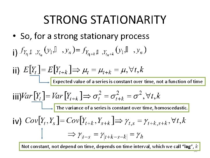
STRONG STATIONARITY • So, for a strong stationary process i) ii) Expected value of a series is constant over time, not a function of time iii) The variance of a series is constant over time, homoscedastic. iv) Not constant, not depend on time, depends on time interval, which we call “lag”, k 36

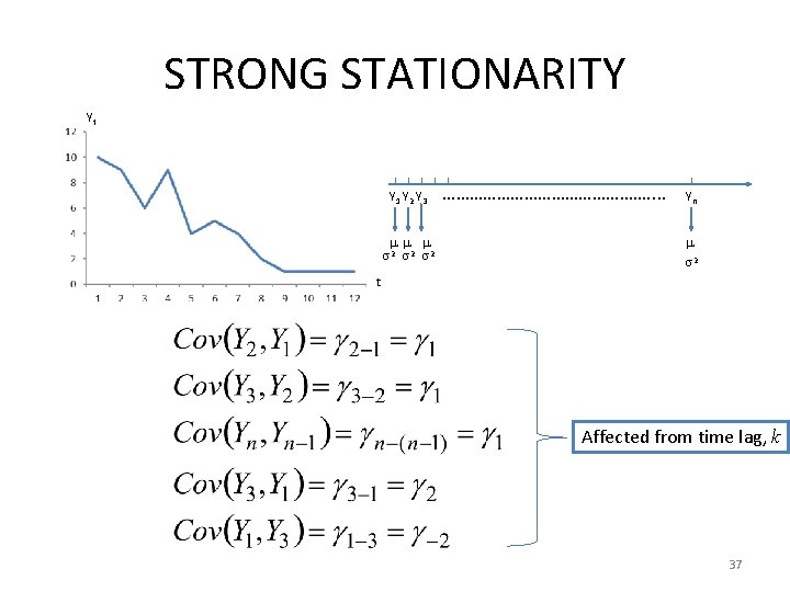
STRONG STATIONARITY Yt Y 1 Y 2 Y 3 2 2 2 ……………………. . Yn 2 t Affected from time lag, k 37

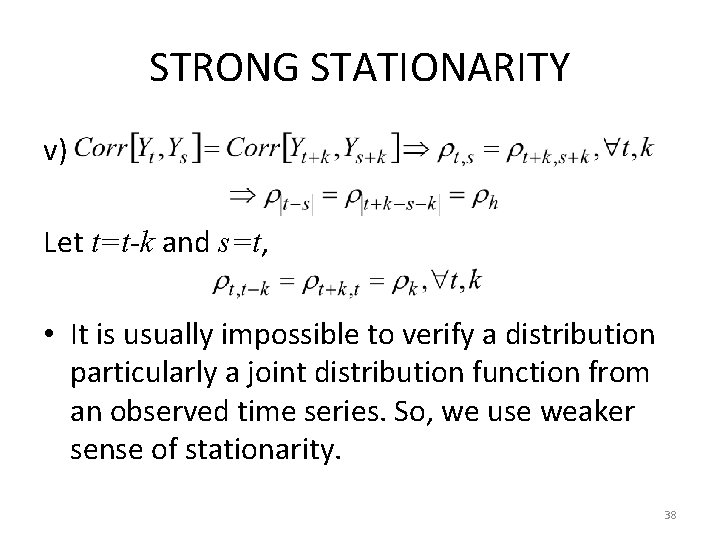
STRONG STATIONARITY v) Let t=t-k and s=t, • It is usually impossible to verify a distribution particularly a joint distribution function from an observed time series. So, we use weaker sense of stationarity. 38

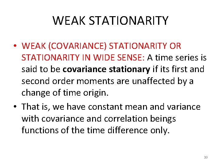
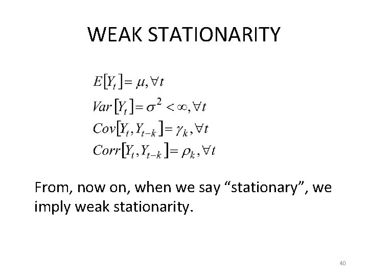
WEAK STATIONARITY • WEAK (COVARIANCE) STATIONARITY OR STATIONARITY IN WIDE SENSE: A time series is said to be covariance stationary if its first and second order moments are unaffected by a change of time origin. • That is, we have constant mean and variance with covariance and correlation beings functions of the time difference only. 39

WEAK STATIONARITY From, now on, when we say “stationary”, we imply weak stationarity. 40

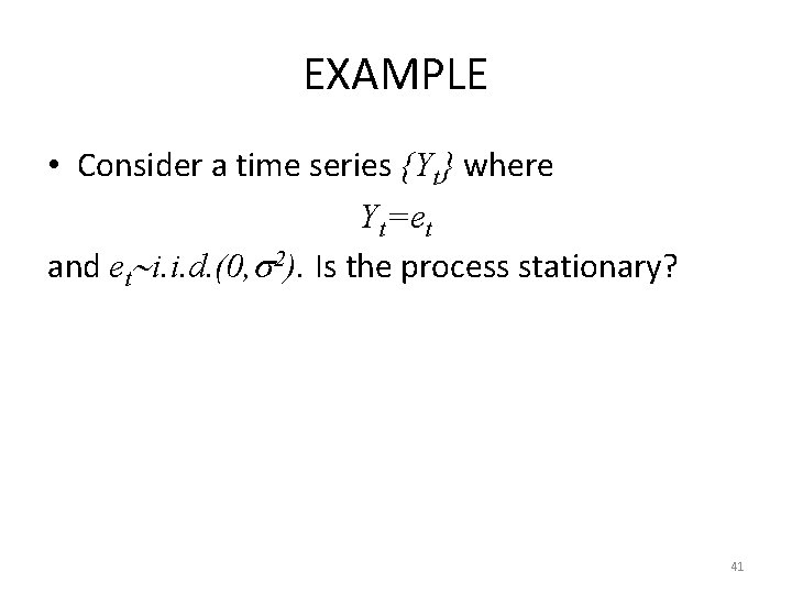
EXAMPLE • Consider a time series {Yt} where Yt=et and et i. i. d. (0, 2). Is the process stationary? 41

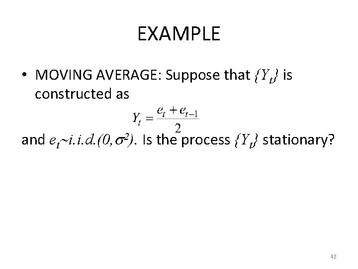
EXAMPLE • MOVING AVERAGE: Suppose that {Yt} is constructed as and et i. i. d. (0, 2). Is the process {Yt} stationary? 42

EXAMPLE • RANDOM WALK where et i. i. d. (0, 2). Is the process {Yt} stationary? 43

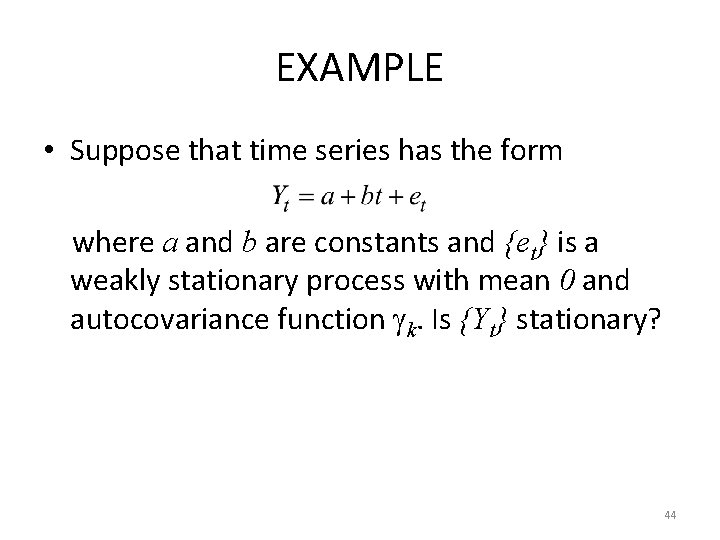
EXAMPLE • Suppose that time series has the form where a and b are constants and {et} is a weakly stationary process with mean 0 and autocovariance function k. Is {Yt} stationary? 44

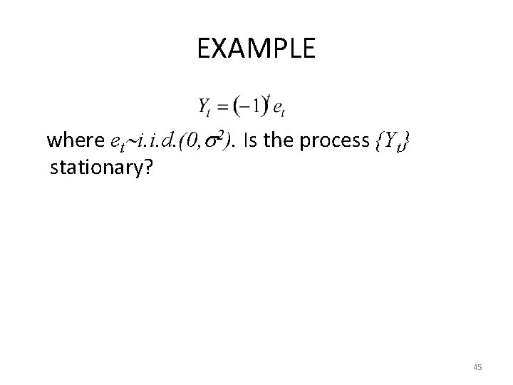
EXAMPLE where et i. i. d. (0, 2). Is the process {Yt} stationary? 45

STRONG VERSUS WEAK STATIONARITY • Strict stationarity means that the joint distribution only depends on the ‘difference’ h, not the time (t 1, . . . , tk). • Finite variance is not assumed in the definition of strong stationarity, therefore, strict stationarity does not necessarily imply weak stationarity. For example, processes like i. i. d. Cauchy is strictly stationary but not weak stationary. • A nonlinear function of a strict stationary variable is still strictly stationary, but this is not true for weak stationary. For example, the square of a covariance stationary process may not have finite variance. • Weak stationarity usually does not imply strict stationarity as higher moments of the process may depend on time t. 46

STRONG VERSUS WEAK STATIONARITY • If process {Xt} is a Gaussian time series, which means that the distribution functions of {Xt} are all multivariate Normal, weak stationary also implies strict stationary. This is because a multivariate Normal distribution is fully characterized by its first two moments. 47

STRONG VERSUS WEAK STATIONARITY • For example, a white noise is stationary but may not be strict stationary, but a Gaussian white noise is strict stationary. Also, general white noise only implies uncorrelation while Gaussian white noise also implies independence. Because if a process is Gaussian, uncorrelation implies independence. Therefore, a Gaussian white noise is just i. i. d. N(0, 2). 48

STATIONARITY AND NONSTATIONARITY • Stationary and nonstationary processes are very different in their properties, and they require different inference procedures. We will discuss this in detail through this course. 49