Time series and Trend analysis A time series

Time series and Trend analysis A time series consists of a set of observations measured at specified, usually equal, time interval. Time series analysis attempts to identify those factors that exert influence on the values in the series.

. Time series analysis is a basic tool forecasting. Industry and government must forecast future activity to make decisions and plans to meet projected changes. An analysis of the trend of the observations is needed to acquire an understanding of the progress of events leading to prevailing conditions.

. The trend is defined as the long term underlying growth movement in a time series. Accurate trend spotting can only be determined if the data are available for a sufficient length of time. Forecasting does not produce definitive results. Forecasters can and do get things wrong from election results and football scores to the weather.

Time series examples • • Sales data Gross national product Share prices $A Exchange rate Unemployment rates Population Foreign debt Interest rates

Time series components Time series data can be broken into these four components: 1. 2. 3. 4. Secular trend Seasonal variation Cyclical variation Irregular variation

Components of Time-Series Data Irregular fluctuations Cyclical Trend 1 2 3 4 5 6 7 8 Seasonal 9 10 11 12 Year Predicting long term trends without smoothing? What could go wrong? Where do you commence your prediction from the bottom of a variation going up or the peak of a variation going down………. . 13

1. Secular Trend This is the long term growth or decline of the series. • In economic terms, long term may mean >10 years • Describes the history of the time series • Uses past trends to make prediction about the future • Where the analyst can isolate the effect of a secular trend, changes due to other causes become clearer

3/08/2008 3/08/2007 3/08/2006 3/08/2005 3/08/2004 3/08/2003 3/08/2002 3/08/2001 3/08/2000 3/08/1999 3/08/1998 3/08/1997 3/08/1996 3/08/1995 3/08/1994 3/08/1993 3/08/1992 3/08/1991 3/08/1990 3/08/1989 3/08/1988 3/08/1987 3/08/1986 3/08/1985 3/08/1984 All Ords 8000 7000 6000 5000 4000 3000 All Ords 2000 1000 0

. Look out While trend estimates are often reliable, in some instances the usefulness of estimates is reduced by: • by a high degree of irregularity in original or seasonally adjusted series or • by abrupt change in the time series characteristics of the original data

$A vs $US during day 1 vote count 2000 US Presidential election • . This graph shows the amazing trend of the $A vs $UA during an 18 hour period on November 8, 2000

2. Seasonal Variation The seasonal variation of a time series is a pattern of change that recurs regularly over time. Seasonal variations are usually due to the differences between seasons and to festive occasions such as Easter and Christmas. Examples include: • Air conditioner sales in Summer • Heater sales in Winter • Flu cases in Winter • Airline tickets for flights during school vacations

Monthly Retail Sales in NSW Retail Department Stores

3. Cyclical variations also have recurring patterns but with a longer and more erratic time scale compared to Seasonal variations. The name is quite misleading because these cycles can be far from regular and it is usually impossible to predict just how long periods of expansion or contraction will be. There is no guarantee of a regularly returning pattern.

Cyclical variation Example include: • • • Floods Wars Changes in interest rates Economic depressions or recessions Changes in consumer spending

Cyclical variation This chart represents an economic cycle, but we know it doesn’t always go like this. The timing and length of each phase is not predictable.

4. Irregular variation An irregular (or random) variation in a time series occurs over varying (usually short) periods. It follows no pattern and is by nature unpredictable. It usually occurs randomly and may be linked to events that also occur randomly. Irregular variation cannot be explained mathematically.

Irregular variation If the variation cannot be accounted for by secular trend, season or cyclical variation, then it is usually attributed to irregular variation. Example include: – – – Sudden changes in interest rates Collapse of companies Natural disasters Sudden shift s in government policy Dramatic changes to the stock market Effect of Middle East unrest on petrol prices

Monthly Value of Building Approvals ACT)

. Now we have considered the 4 time series components: 1. 2. 3. 4. Secular trend Seasonal variation Cyclical variation Irregular variation We now take a closer look at secular trends and 5 techniques available to measure the underlying trend.

Why examine the trend? When a past trend can be reasonably expected to continue on, it can be used as the basis of future planning: • Capacity planning for increased population • Utility loads • Market progress

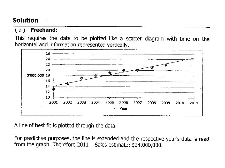
Measure underlying trend freehand graph (plot)

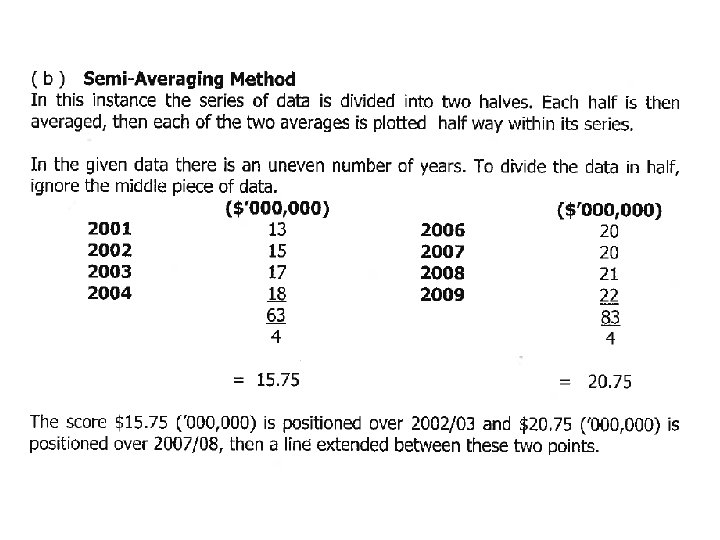
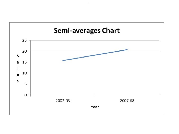
Measure underlying trend Semi-averages This technique attempts to fit a straight line to describe the secular trend: i. Divide data into 2 equal time ranges ii. Calculate the average of the observations in each of the 2 time ranges iii. Draw a straight line between the 2 points iv. Extend line slightly past the end of the original observation to make predictions for future years

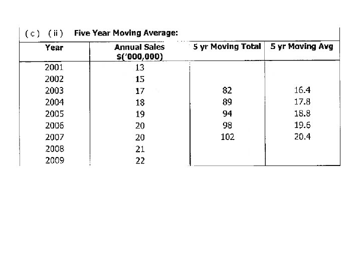
Measure underlying trend Moving averages This method is based on the premise that if values in a time series are averaged over a sufficient period, the effect of short term variations will be reduced. That is, short term, cyclical, seasonal and irregular variations will be smoothed out resulting in an apparently smooth graph depicting the overall trend. The degree of smoothing can be controlled by selecting the number of cases to be included in an average.

The technique for finding a moving average for a particular observation is to find the average of the m observations before and after the observation itself. That is, a total of (2 m + 1 ) observations must be averaged each time a moving average is calculated. Find: both 3 and 5 year moving averages (or mean smoothing) for this time series: Year 2001 2002 2003 2004 2005 2006 2007 2008 2009 Sales 13 15 17 18 19 20 20 21 22

13 + 15 +17 = 45 15 + 17 + 18 = 50…. Or 45 +18 - 13 = 50 (pick up the new drop off the old)

13 + 15 + 17 + 18 = 63, 63 / 4 = 15. 75 + 17. 25 = 33 …… 33 / 2 = 16. 5

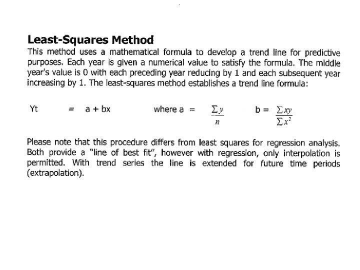
Measure underlying trend Least squares linear regression A more sophisticated way to of fitting a straight line to a time series is to use the method of least squares regression. Sound familiar? The observations are the dependant y variables and time is the independent x variable.

Least squares regression example Soft Drink Sales $’ 000 for Carbonated Pty Ltd Year 2003 2004 2005 2006 2007 2008 2009 2010 2011 Y 13 15 17 18 19 20 20 21 22 165 x x^2 xy

Calculation for least squares regression example.

Least squares regression line. Yt = 18. 3 + 1. 03 x What is the predicted Sales figure for 2013? Hint: what value is x in 2013?

. Yt = 18. 3 + 1. 03 x What is the predicted Sales figure for 2013? Hint: what value is x in 2013? If 2011 = 4, then 2013 = 6, so 6 2 nd f ( = 24. 53

A quick recap….

Line of Best Fit – plot points then draw a line that can be adjusted by clicking either end of the line

Semi Averaging Method at 2002 -3 = 15. 75 and 2007 -8 = 20. 75

Moving Averages (or mean smoothing)

The following 2 slides should be reviewed at home (with strong coffee) …

Measure underlying trend – exponential smoothing

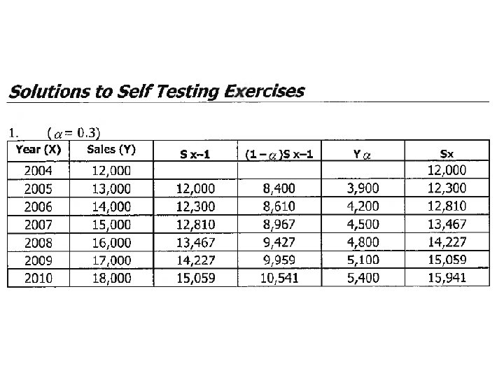
. The trend line is calculated using this formula where: • Sx = the smoothed value for observation x • Y = the actual value of observation x • Sx-1 = the smoothed value previously calculated for observation (x-1) • =the smoothing constant where 0 1

. The exponential smoothing approach has to have a starting point, so we choose the first smoothed value (S 1) to be the first observation (Y 1) in the time series. The smoothed value of each observation is a function of the smoothed value of the observation immediately before it. Errors made in calculating the smoothed values will carry on for each successive time period.

Exponential smoothing = 0. 4 Year Sales (Y) Sx-1 (1 - ) Sx-1 Y Sx 2004 12, 000 2005 12, 500 12, 000 7, 200 5, 000 2006 12, 200 4, 880 2007 13, 000 5, 2008 13, 500 5, 400 2009 13, 400 5, 360 2010 14, 000 5, 600

Complete the table below 2005 - 12500 x. 4 = 5000 , 12000 x. 6 = 7200, then Sx = 7200 + 5000 = 12200 Bring Sx figure down to Sx-1 for start of 2006 (figure is 12200) 2006 - 12200 x. 4 = 4880, 12200 x. 6 = 7320 , Sx = 4880 + 7320 = 12200 2007 - Sx-1 = 12200, 13000 x. 4 = 5200, 12200 x. 6=7320 , Sx = 5200+7320 = 12520 2008 - Sx-1 = 12520, 13500 x. 4=5400, 12520 x. 6=7512, etc.

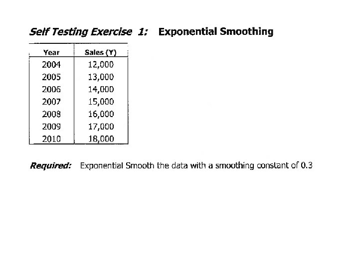
Self testing exercise 1 = 0. 3

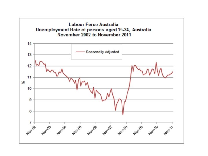
The ABS has some useful information on Seasonal Data

. A seasonally adjusted series involves estimating and removing the cyclical and seasonal effects from the original data. Seasonally adjusting a time series is useful if you wish to understand the underlying patterns of change or movement in a population, without the impact of the seasonal or cyclical effects. For example, employment and unemployment are often seasonally adjusted so that the actual change in employment and unemployment levels can be seen, without the impact of periods of peak employment such as Christmas/New Year when a large number of casual workers are temporarily employed.

. Suppose there were some adverse publicity in December about ice-cream. It would be incorrect simply to compare the sales of ice -cream in June with those in December to determine the effect of the bad publicity. December would have higher sales in any case, because it is warmer. Useful comparisons of sales could only be made after seasonal variation had been allowed for. The true impact of the publicity could then be determined.

Show “D = A / Si” can be re-arranged to be Si = A / D – memory trigger the word “SAID” except the I is the division symbol or the word “DAISY” with “I” as the division symbol

You tube clip calculating Seasonal indices http: //www. youtube. com/watch? v=7 Ug 2 z. A 0 M-1 Y&feature=related

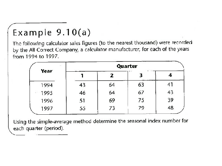
SI - simple average method The simple average method takes the average for each period (period mean) over a period of at least three years, and expresses that as an index by comparing it to the average of all periods over the same period of time. Note: indices can be based on periods such as months or weeks.

Yearly average 1994 = 43 + 64 + 63 + 41 = 211/4 = 52. 75 Yearly average 1995 = 46 + 64 + 67 + 43 = 220 /4 = 55. 0 Yearly average 1996= 51 + 69 + 75 + 39 = 234/4 = 58. 5 Yearly average 1997= 55 + 73 + 79 + 48 = 255 / 4 =63. 75

. To calculate quarterly SI using same technique as video: 1994 Q 1 Seasonal Index is 1994 Q 1 sales/ average for 1994 = 43 / 52. 75 = 0. 82 Q 1 Q 2 Q 3 Q 4 1994 0. 82 1. 21 1. 19 0. 78 1995 0. 84 1. 16 1. 22 0. 78 1996 0. 87 1. 18 1. 28 0. 67 1997 0. 86 1. 15 1. 24 0. 75 total 3. 39 4. 70 4. 93 2. 98

. total 3. 39 4. 70 4. 93 2. 98 Divide by 4 0. 85 1. 18 1. 23 0. 75 to get SI

Alternate approach to calculate Seasonal Index number for each quarter note: same result!

D = A / SI x 100 60 = 51 / 84. 8 x 100

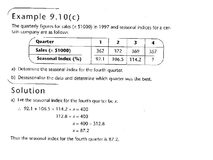
D = A / SI x 100 393 = 362 / 92. 1 x 100 So even though Actual sales in the 4 th quarter were $357 – once we take the seasonal factor out of the equation we can see it was the best performing quarter.

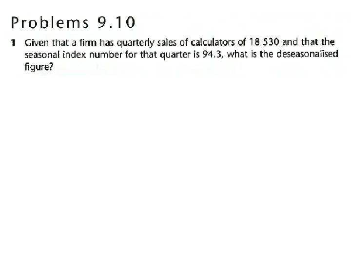
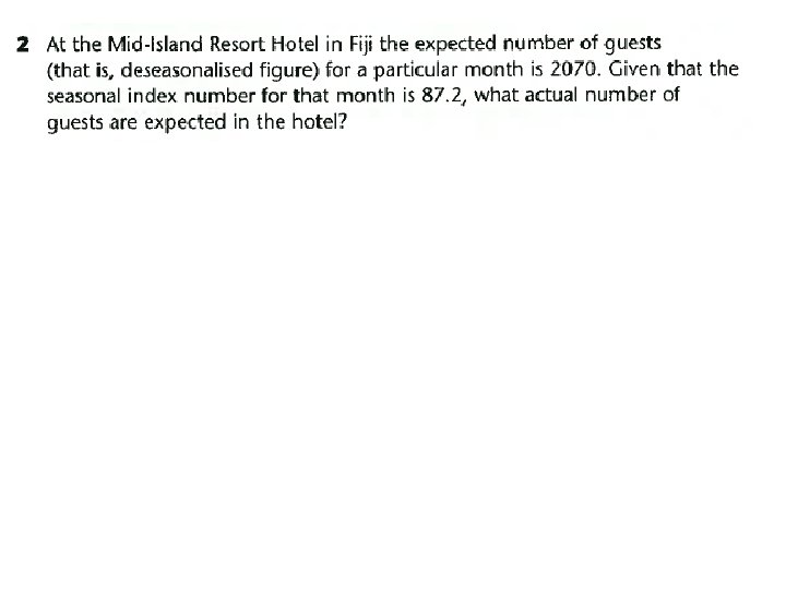
Projected figures will always be performed on deseasonalised figures D = A / SI x 100 Therefore A = D x SI / 100

D = A / SI x 100 D = 18530 / 94. 3 x 100 = 19650

D = A / SI x 100 Therefore A = D x SI / 100 A = 2070 x 87. 2 / 100 = 1805

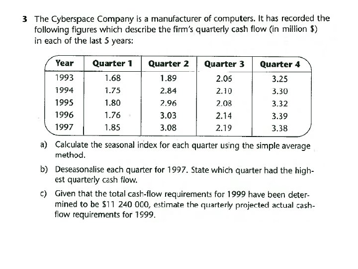
Quarter 1 = 1. 68 + 1. 75 + 1. 80 + 1. 76 + 1. 85 = 8. 84 / 5 = 1. 768 Quarter 2 = 1. 89 + 2. 84 + 2. 96 +3. 03 + 3. 08 = 13. 8 / 5 = 2. 76 Quarter 3 = 2. 06 + 2. 1 + 2. 08 + 2. 14 +2. 19 = 10. 57 / 5 = 2. 114 Quarter 4 = 3. 25 + 3. 32 + 3. 39 + 3. 38 = 16. 64 / 5 = 3. 328 Average for the quarters = 1. 768 + 2. 76 + 2. 114 + 3. 328 = 9. 97 / 4 = 2. 4925 Index for Quarter 1 = 1. 768 / 2. 4925 x 100 = 70. 93

D = A / SI x 100 1997 Quarter 1 = D = 1. 85 / 70. 93 x 100 = 2. 61

11. 24 / 4 = Quarterly deseasonalised data = 2. 81 D = A / SI x 100 Therefore A = D x SI / 100 Quarter 1 = A = 2. 81 x 70. 93 / 100 = 1. 99