The Properties of Time Series Lecture 4 Previously

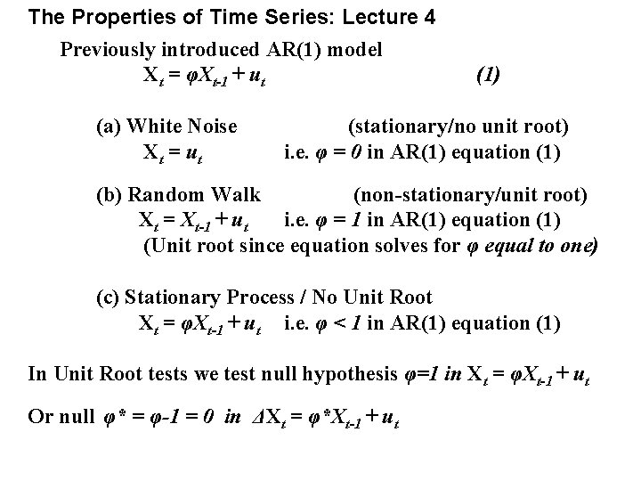
The Properties of Time Series: Lecture 4 Previously introduced AR(1) model Xt = φXt-1 + ut (a) White Noise Xt = ut (1) (stationary/no unit root) i. e. φ = 0 in AR(1) equation (1) (b) Random Walk (non-stationary/unit root) Xt = Xt-1 + ut i. e. φ = 1 in AR(1) equation (1) (Unit root since equation solves for φ equal to one) (c) Stationary Process / No Unit Root Xt = φXt-1 + ut i. e. φ < 1 in AR(1) equation (1) In Unit Root tests we test null hypothesis φ=1 in Xt = φXt-1 + ut Or null φ* = φ-1 = 0 in ΔXt = φ*Xt-1 + ut

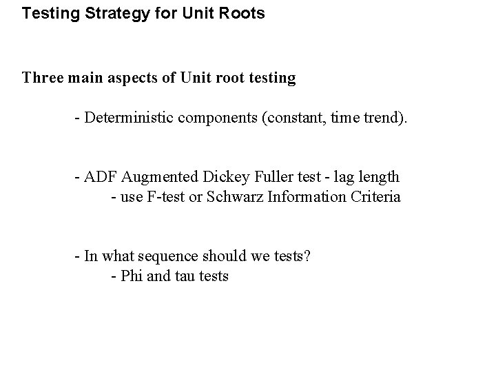
Testing Strategy for Unit Roots Three main aspects of Unit root testing - Deterministic components (constant, time trend). - ADF Augmented Dickey Fuller test - lag length - use F-test or Schwarz Information Criteria - In what sequence should we tests? - Phi and tau tests

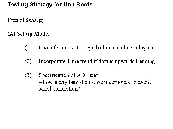
Testing Strategy for Unit Roots Formal Strategy (A) Set up Model (1) Use informal tests – eye ball data and correlogram (2) Incorporate Time trend if data is upwards trending (3) Specification of ADF test – how many lags should we incorporate to avoid serial correlation?

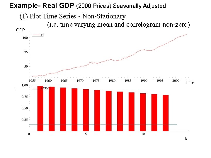
Example- Real GDP (2000 Prices) Seasonally Adjusted (1) Plot Time Series - Non-Stationary (i. e. time varying mean and correlogram non-zero) GDP Time r k

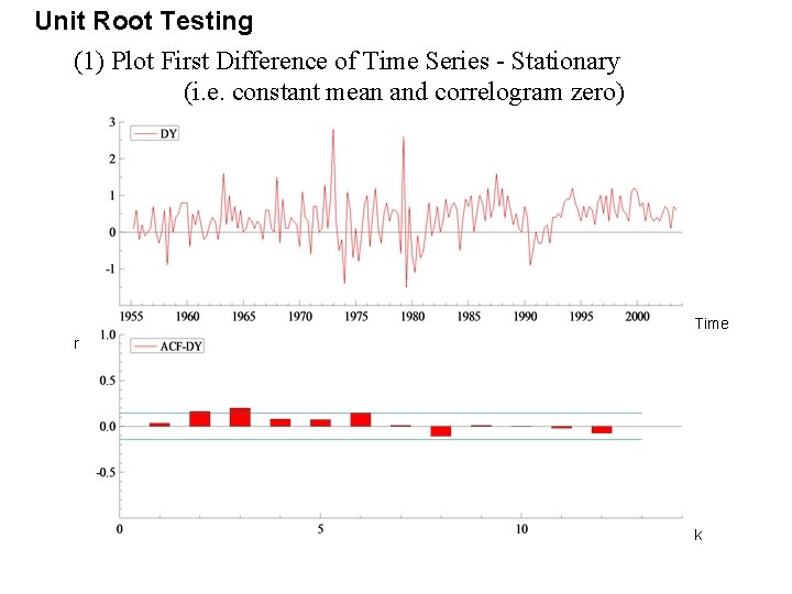
Unit Root Testing (1) Plot First Difference of Time Series - Stationary (i. e. constant mean and correlogram zero) Time r k

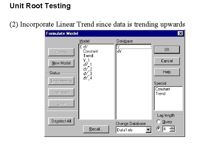
Unit Root Testing (2) Incorporate Linear Trend since data is trending upwards

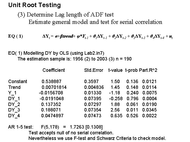
Unit Root Testing (3) Determine Lag length of ADF test Estimate general model and test for serial correlation EQ ( 1) ΔYt = α+βtrend+ φ*Yt-1 + θ 1ΔYt-1 + θ 2ΔYt-2 + θ 3ΔYt-3 + θ 4ΔYt-4 + ut EQ( 1) Modelling DY by OLS (using Lab 2. in 7) The estimation sample is: 1956 (2) to 2003 (3) n = 190 Constant Trend Y_1 DY_2 DY_3 DY_4 Coefficient Std. Error t-value t-prob Part. R^2 0. 538887 0. 00701814 -0. 0156708 -0. 0191048 0. 137352 0. 188071 0. 0474897 0. 3597 0. 004836 0. 01330 0. 07395 0. 07297 0. 07354 0. 07473 1. 50 1. 45 -1. 18 -0. 258 1. 88 2. 56 0. 635 0. 136 0. 148 0. 240 0. 796 0. 061 0. 011 0. 526 0. 0121 0. 0114 0. 0075 0. 0004 0. 0190 0. 0345 0. 0022 AR 1 -5 test: F(5, 178) = 1. 7263 [0. 1308] Test accepts null of no serial correlation. Nevertheless we use F-test and Schwarz Criteria to check model.

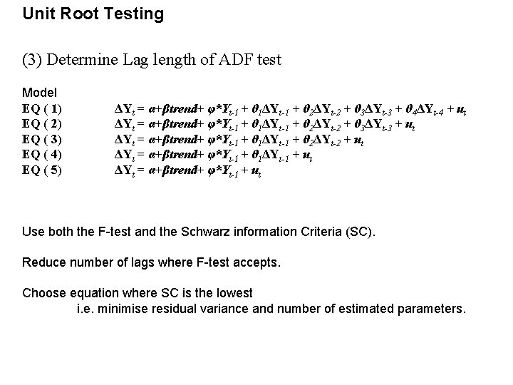
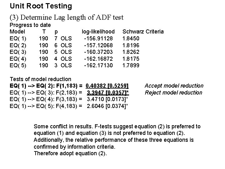
Unit Root Testing (3) Determine Lag length of ADF test Model EQ ( 1) EQ ( 2) EQ ( 3) EQ ( 4) EQ ( 5) ΔYt = α+βtrend+ φ*Yt-1 + θ 1ΔYt-1 + θ 2ΔYt-2 + θ 3ΔYt-3 + θ 4ΔYt-4 + ut ΔYt = α+βtrend+ φ*Yt-1 + θ 1ΔYt-1 + θ 2ΔYt-2 + θ 3ΔYt-3 + ut ΔYt = α+βtrend+ φ*Yt-1 + θ 1ΔYt-1 + θ 2ΔYt-2 + ut ΔYt = α+βtrend+ φ*Yt-1 + θ 1ΔYt-1 + ut ΔYt = α+βtrend+ φ*Yt-1 + ut Use both the F-test and the Schwarz information Criteria (SC). Reduce number of lags where F-test accepts. Choose equation where SC is the lowest i. e. minimise residual variance and number of estimated parameters.

Unit Root Testing (3) Determine Lag length of ADF test Progress to date Model T EQ( 1) 190 EQ( 2) 190 EQ( 3) 190 EQ( 4) 190 EQ( 5) 190 p 7 6 5 4 3 OLS OLS OLS log-likelihood -156. 91128 -157. 12068 -160. 37203 -162. 16872 -162. 17130 Tests of model reduction EQ( 1) --> EQ( 2): F(1, 183) = EQ( 1) --> EQ( 3): F(2, 183) = EQ( 1) --> EQ( 4): F(3, 183) = EQ( 1) --> EQ( 5): F(4, 183) = Schwarz Criteria 1. 8450 1. 8196 1. 8262 1. 8175 1. 7899 0. 40382 [0. 5259] 3. 3947 [0. 0357]* 3. 4710 [0. 0173]* 2. 6046 [0. 0374]* Accept model reduction Reject model reduction Some conflict in results. F-tests suggest equation (2) is preferred to equation (1) and equation (3) is not preferred to equation (2). Additionally, the relative performance of these three equations is confirmed by information criteria. Therefore adopt equation (2).

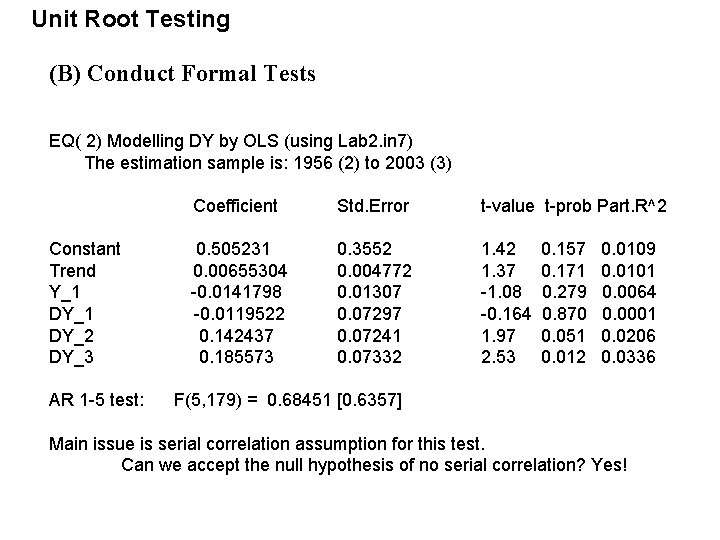
Unit Root Testing (B) Conduct Formal Tests EQ( 2) Modelling DY by OLS (using Lab 2. in 7) The estimation sample is: 1956 (2) to 2003 (3) Constant Trend Y_1 DY_2 DY_3 AR 1 -5 test: Coefficient Std. Error t-value t-prob Part. R^2 0. 505231 0. 00655304 -0. 0141798 -0. 0119522 0. 142437 0. 185573 0. 3552 0. 004772 0. 01307 0. 07297 0. 07241 0. 07332 1. 42 1. 37 -1. 08 -0. 164 1. 97 2. 53 0. 157 0. 171 0. 279 0. 870 0. 051 0. 012 0. 0109 0. 0101 0. 0064 0. 0001 0. 0206 0. 0336 F(5, 179) = 0. 68451 [0. 6357] Main issue is serial correlation assumption for this test. Can we accept the null hypothesis of no serial correlation? Yes!

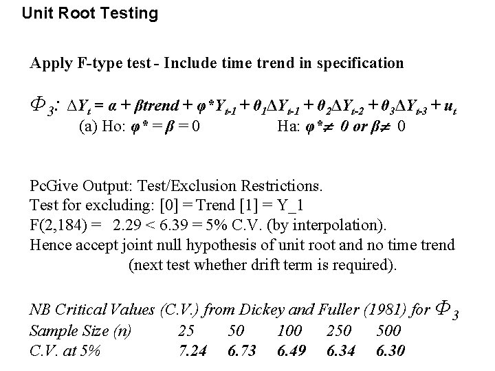
Unit Root Testing Apply F-type test - Include time trend in specification Φ 3: ΔYt = α + βtrend + φ*Yt-1 + θ 1ΔYt-1 + θ 2ΔYt-2 + θ 3ΔYt-3 + ut (a) Ho: φ* = β = 0 Ha: φ* 0 or β 0 Pc. Give Output: Test/Exclusion Restrictions. Test for excluding: [0] = Trend [1] = Y_1 F(2, 184) = 2. 29 < 6. 39 = 5% C. V. (by interpolation). Hence accept joint null hypothesis of unit root and no time trend (next test whether drift term is required). NB Critical Values (C. V. ) from Dickey and Fuller (1981) for Φ 3 Sample Size (n) 25 50 100 250 500 C. V. at 5% 7. 24 6. 73 6. 49 6. 34 6. 30

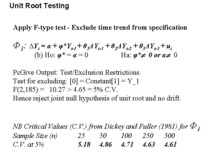
Unit Root Testing Apply F-type test - Exclude time trend from specification Φ 1: ΔYt = α + φ*Yt-1 + θ 1ΔYt-1 + θ 2ΔYt-2 + θ 3ΔYt-3 + ut (b) Ho: φ* = α = 0 Ha: φ* 0 or α 0 Pc. Give Output: Test/Exclusion Restrictions. Test for excluding: [0] = Constant[1] = Y_1 F(2, 185) = 10. 27 > 4. 65 = 5% C. V. Hence reject joint null hypothesis of unit root and no drift. NB Critical Values (C. V. ) from Dickey and Fuller (1981) for Φ 1 Sample Size (n) 25 50 100 250 500 C. V. at 5% 5. 18 4. 86 4. 71 4. 63 4. 61

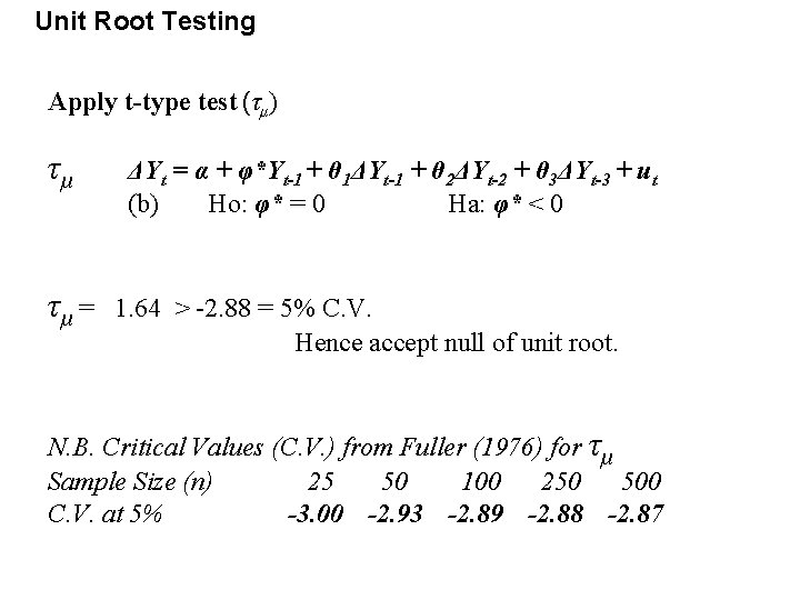
Unit Root Testing Apply t-type test (τμ) τμ τμ = ΔYt = α + φ*Yt-1 + θ 1ΔYt-1 + θ 2ΔYt-2 + θ 3ΔYt-3 + ut (b) Ho: φ* = 0 Ha: φ* < 0 1. 64 > -2. 88 = 5% C. V. Hence accept null of unit root. N. B. Critical Values (C. V. ) from Fuller (1976) for τμ Sample Size (n) 25 50 100 250 500 C. V. at 5% -3. 00 -2. 93 -2. 89 -2. 88 -2. 87

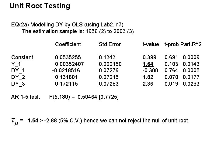
Unit Root Testing EQ(2 a) Modelling DY by OLS (using Lab 2. in 7) The estimation sample is: 1956 (2) to 2003 (3) Constant Y_1 DY_2 DY_3 AR 1 -5 test: τμ = Coefficient Std. Error t-value t-prob Part. R^2 0. 0535255 0. 00352407 -0. 0218516 0. 131601 0. 172115 0. 1343 0. 002150 0. 07279 0. 07215 0. 07283 0. 399 1. 64 -0. 300 1. 82 2. 36 0. 691 0. 103 0. 764 0. 070 0. 019 0. 0009 0. 0143 0. 0005 0. 0177 0. 0293 F(5, 180) = 0. 50464 [0. 7725] 1. 64 > -2. 88 (5% C. V. ) hence we can not reject the null of unit root.

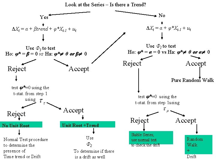
Look at the Series – Is there a Trend? No Yes ΔXt = α + φ*Xt-1 + ut ΔXt = α + βtrend + φ*Xt-1 + ut Use Φ 3 to test Ho: φ* = β = 0 vs Ha: φ* 0 or β 0 Reject Accept Use Φ 1 to test Ho: φ* = α = 0 vs Ha: φ* 0 or α 0 Reject Accept Pure Random Walk test φ*=0 using the t-stat. from step 1 using Reject No Unit Root Normal Test procedure to determine the presence of Time trend or Drift test φ*=0 using the t-stat. from step 1 using Accept Unit Root +Trend Use Φ 2 To determine if there is a drift as well Reject Stable Series, use normal test to check the drift Accept Random Walk + Drift

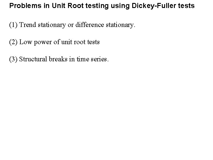
Problems in Unit Root testing using Dickey-Fuller tests (1) Trend stationary or difference stationary. (2) Low power of unit root tests (3) Structural breaks in time series.

Problems in Unit root testing (1) Trend Stationary Process and Difference Stationary Process. Graph of GDP could be approximated by linear trend - Nelson and Plosser (1982) challenged this assumption trend was a random walk for many series. - Trend was not fixed but was moved by random shocks, and would stay as such until hit by another shock. This problem can be resolved partially by careful application of F-type tests. - e. g. from before there is no evidence of trend for Φ 3

Problems in Unit root testing (2) Low power of unit root tests - Is φ* = 0 in ΔXt = α + φ*Xt-1 + ut Test result is based on the standard error of φ* - Measure of how accurate is our estimated coefficient - with increasing observations we become more certain. Power of a tests is ability to reject the null when it is false. e. g. ability to accept alternative hypothesis of stationarity. Low power implies a series may be stationary but Dickey. Fuller test suggests unit root. - low power is especially a problem when series is stationary but close to being unit root.

Problems in Unit root testing One solution to low power is to increase the number of observations by increasing the span of data. However, there may be differences in economic structure or policy which should be modelled differently. (3) Structural breaks in time series. - Perron (1989): movement of trend could be explained by single break. - Nelson-Plosser series are not random walk but linear trend with single breaks. Alternative solution to low power is a number of joint ADF tests. - Take information from a number of countries. - And pool coefficients. (i. e. combine information).