Dimensionality Reduction UV Decomposition SingularValue Decomposition CUR Decomposition

Dimensionality Reduction UV Decomposition Singular-Value Decomposition CUR Decomposition Jeffrey D. Ullman Stanford University

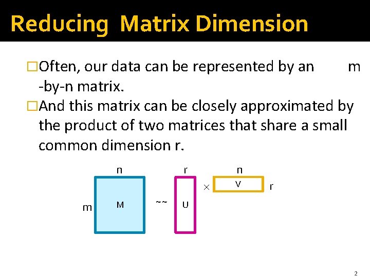
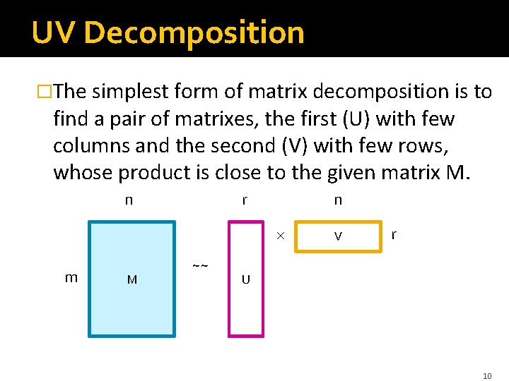
Reducing Matrix Dimension �Often, our data can be represented by an m -by-n matrix. �And this matrix can be closely approximated by the product of two matrices that share a small common dimension r. m M n r n ~~ V r U 2

Why Is That Even Possible? �There are hidden, or latent factors that – to a close approximation – explain why the values are as they appear in the matrix. �Two kinds of data may exhibit this behavior: 1. Matrices representing a many-relationship. 2. Matrices that are really a relation (as in a relational database). 3

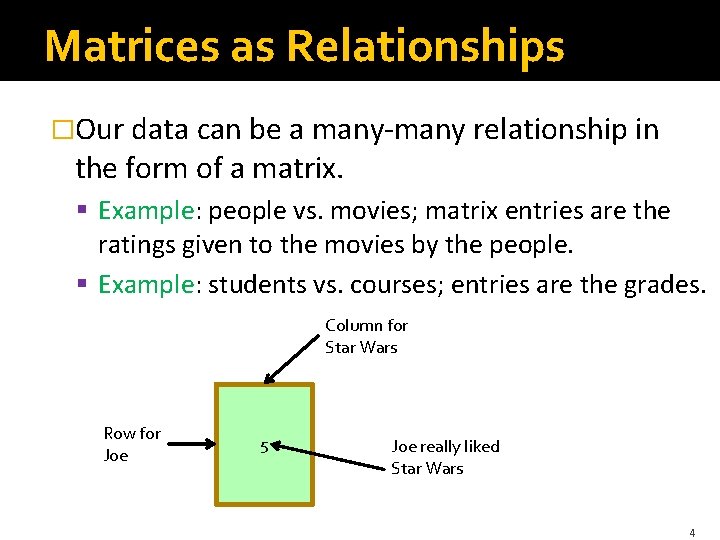
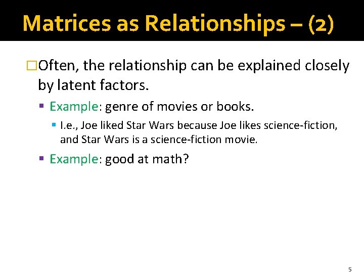
Matrices as Relationships �Our data can be a many-many relationship in the form of a matrix. § Example: people vs. movies; matrix entries are the ratings given to the movies by the people. § Example: students vs. courses; entries are the grades. Column for Star Wars Row for Joe 5 Joe really liked Star Wars 4

Matrices as Relationships – (2) �Often, the relationship can be explained closely by latent factors. § Example: genre of movies or books. § I. e. , Joe liked Star Wars because Joe likes science-fiction, and Star Wars is a science-fiction movie. § Example: good at math? 5

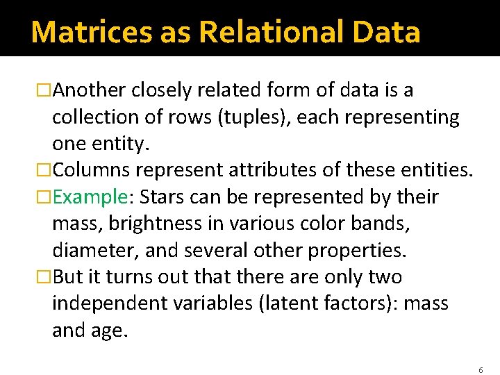
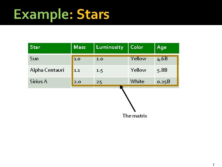
Matrices as Relational Data �Another closely related form of data is a collection of rows (tuples), each representing one entity. �Columns represent attributes of these entities. �Example: Stars can be represented by their mass, brightness in various color bands, diameter, and several other properties. �But it turns out that there are only two independent variables (latent factors): mass and age. 6

Example: Stars Star Mass Luminosity Color Age Sun 1. 0 Yellow 4. 6 B Alpha Centauri 1. 1 1. 5 Yellow 5. 8 B Sirius A 2. 0 25 White 0. 25 B The matrix 7

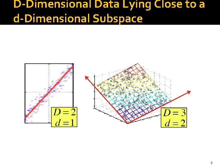
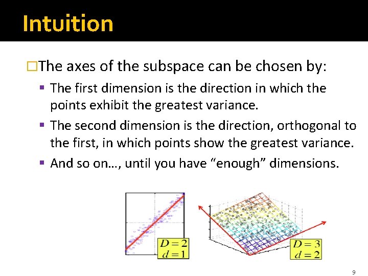
D-Dimensional Data Lying Close to a d-Dimensional Subspace 8

Intuition �The axes of the subspace can be chosen by: § The first dimension is the direction in which the points exhibit the greatest variance. § The second dimension is the direction, orthogonal to the first, in which points show the greatest variance. § And so on…, until you have “enough” dimensions. 9

UV Decomposition �The simplest form of matrix decomposition is to find a pair of matrixes, the first (U) with few columns and the second (V) with few rows, whose product is close to the given matrix M. n n r m M ~~ V r U 10

Latent Factors �This decomposition works well if r is the number of “hidden factors’’ that explain the matrix M. �Example: mij is the rating person i gives to movie j; uik measures how much person i likes genre k; vkj measures the extent to which movie j belongs to genre k. 11

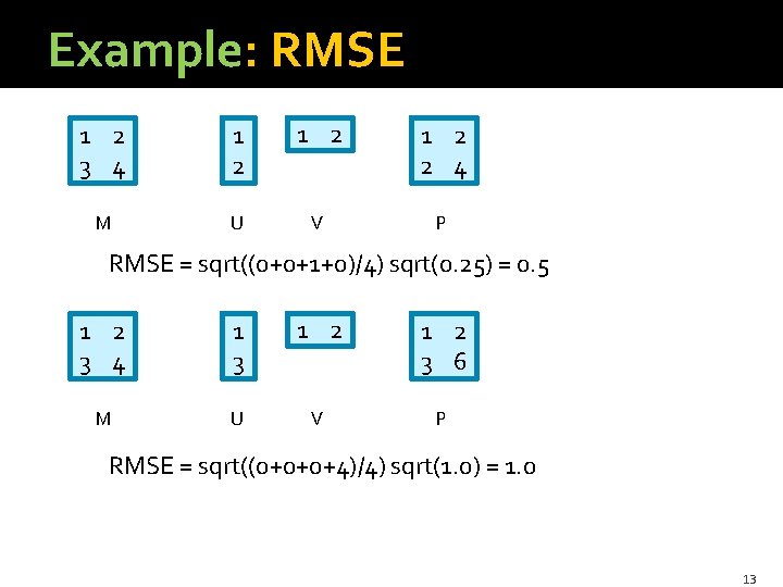
Measuring the Error �Common way to evaluate how well P = UV approximates M is by RMSE (root-mean-square error). �Average (mij – pij)2 over all i and j. �Take the square root. § Square-rooting changes the scale of error, but doesn’t really effect which choice of U and V is best. 12

Example: RMSE 1 2 3 4 1 2 1 2 2 4 M U V P RMSE = sqrt((0+0+1+0)/4) sqrt(0. 25) = 0. 5 1 2 3 4 1 3 1 2 3 6 M U V P RMSE = sqrt((0+0+0+4)/4) sqrt(1. 0) = 1. 0 13

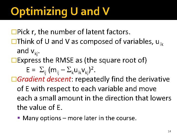
Optimizing U and V �Pick r, the number of latent factors. �Think of U and V as composed of variables, uik and vkj. �Express the RMSE as (the square root of) E = ij (mij – kuikvkj)2. �Gradient descent: repeatedly find the derivative of E with respect to each variable and move each a small amount in the direction that lowers the value of E. § Many options – more later in the course. 14

Local Versus Global Minima �Expressions like this usually have many minima. �Seeking the nearest minimum from a starting point can trap you in a local minimum, from which no small improvement is possible. But you can get trapped here Global minimum 15

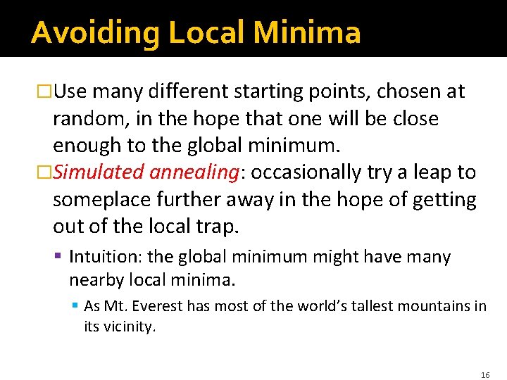
Avoiding Local Minima �Use many different starting points, chosen at random, in the hope that one will be close enough to the global minimum. �Simulated annealing: occasionally try a leap to someplace further away in the hope of getting out of the local trap. § Intuition: the global minimum might have many nearby local minima. § As Mt. Everest has most of the world’s tallest mountains in its vicinity. 16

Application: Recommendations �UV decomposition can be used even when the entire matrix M is not known. �Example: recommendation systems, where M represents known ratings of movies (e. g. ) by people. �Jure will cover recommendation systems next week. 17

Singular-Value Decomposition Rank of a Matrix Orthonormal Bases Eigenvalues/Eigenvectors Computing the Decomposition Eliminating Dimensions

Why SVD? �Gives a decomposition of any matrix into a product of three matrices. �There are strong constraints on the form of each of these matrices. § Results in a decomposition that is essentially unique. �From this decomposition, you can choose any number r of intermediate concepts (latent factors) in a way that minimizes the RMSE error given that value of r. 19

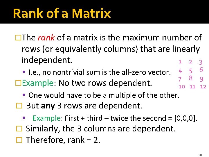
Rank of a Matrix �The rank of a matrix is the maximum number of rows (or equivalently columns) that are linearly independent. 1 2 3 § I. e. , no nontrivial sum is the all-zero vector. 4 5 6 �Example: No two rows dependent. 7 8 9 10 11 12 § One would have to be a multiple of the other. � But any 3 rows are dependent. § Example: First + third – twice the second = [0, 0, 0]. � � Similarly, the 3 columns are dependent. Therefore, rank = 2. 20

Important Fact About Rank �If a matrix has rank r, then it can be decomposed exactly into matrices whose shared dimension is r. �Example, in Sect. 11. 3 of MMDS, of a 7 -by-5 matrix with rank 2 and an exact decomposition into a 7 -by-2 and a 2 -by-5 matrix. 21

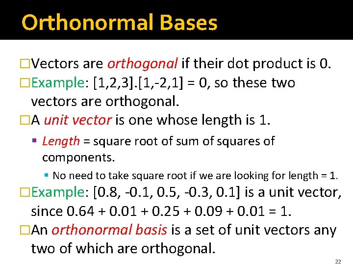
Orthonormal Bases �Vectors are orthogonal if their dot product is 0. �Example: [1, 2, 3]. [1, -2, 1] = 0, so these two vectors are orthogonal. �A unit vector is one whose length is 1. § Length = square root of sum of squares of components. § No need to take square root if we are looking for length = 1. �Example: [0. 8, -0. 1, 0. 5, -0. 3, 0. 1] is a unit vector, since 0. 64 + 0. 01 + 0. 25 + 0. 09 + 0. 01 = 1. �An orthonormal basis is a set of unit vectors any two of which are orthogonal. 22

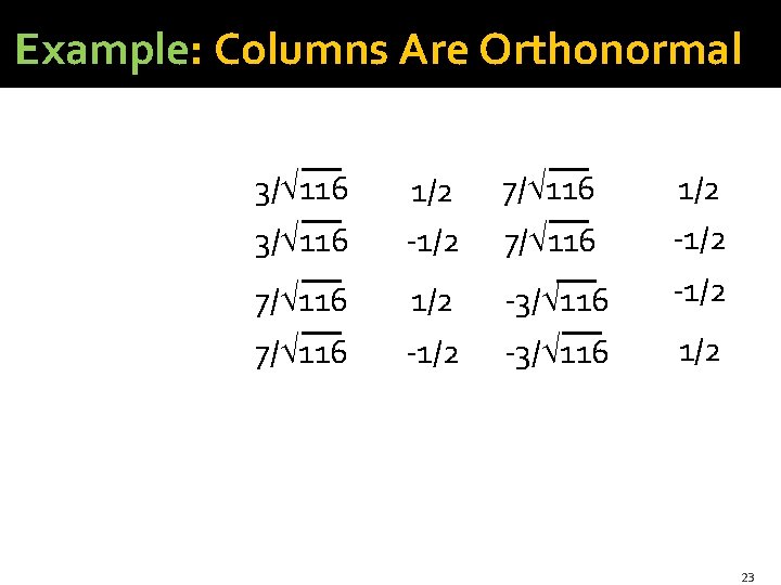
Example: Columns Are Orthonormal 3/ 116 1/2 -1/2 7/ 116 1/2 -3/ 116 -1/2 7/ 116 -1/2 -3/ 116 1/2 23

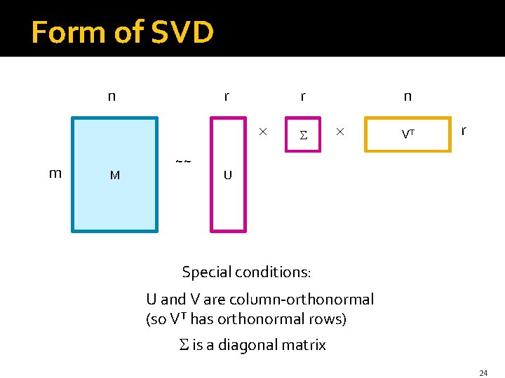
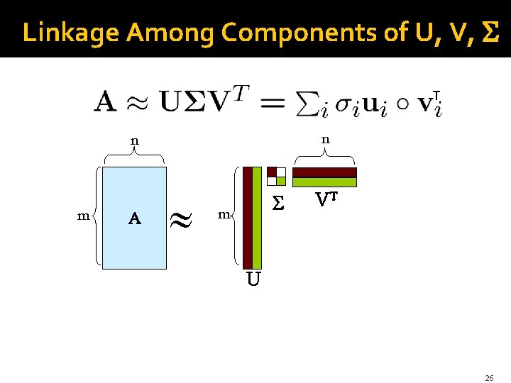
Form of SVD n r m M ~~ n r VT r U Special conditions: U and V are column-orthonormal (so VT has orthonormal rows) is a diagonal matrix 24

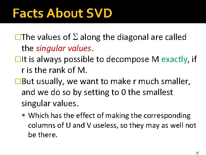
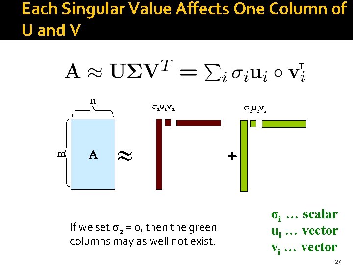
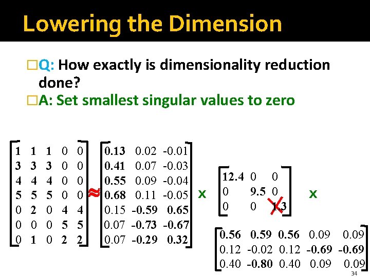
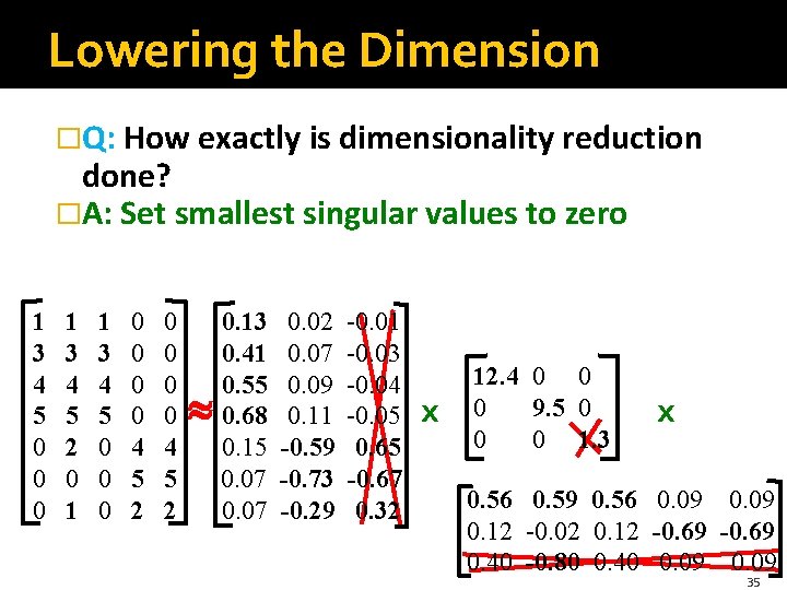
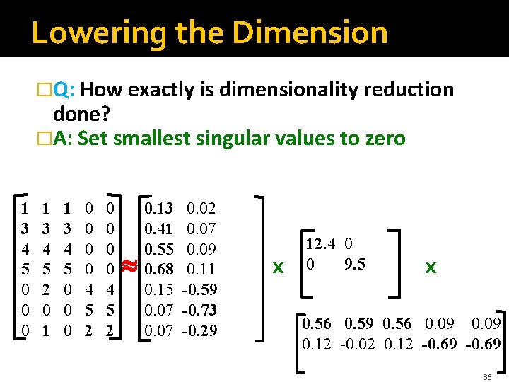
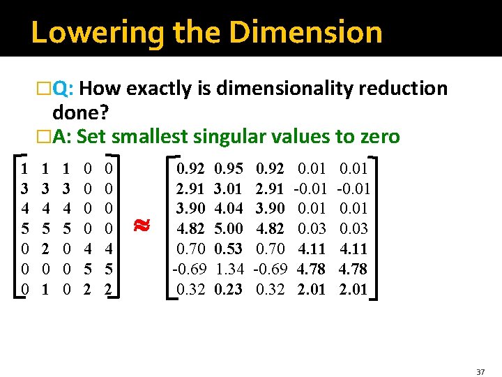
Facts About SVD �The values of along the diagonal are called the singular values. �It is always possible to decompose M exactly, if r is the rank of M. �But usually, we want to make r much smaller, and we do so by setting to 0 the smallest singular values. § Which has the effect of making the corresponding columns of U and V useless, so they may as well not be there. 25

Linkage Among Components of U, V, T n n m A m VT U 26

Each Singular Value Affects One Column of U and V T n m A 1 u 1 v 1 If we set 2 = 0, then the green columns may as well not exist. 2 u 2 v 2 + σi … scalar ui … vector vi … vector 27

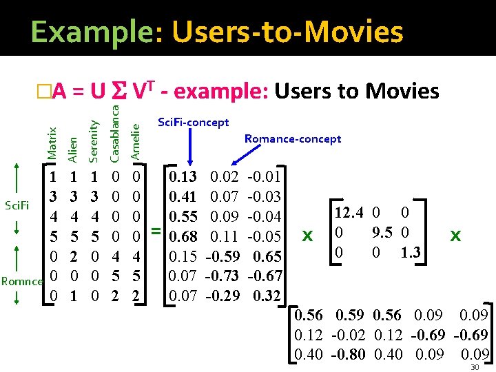
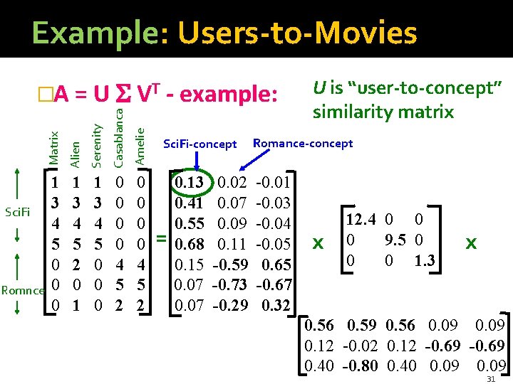
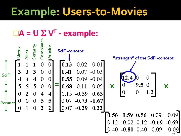
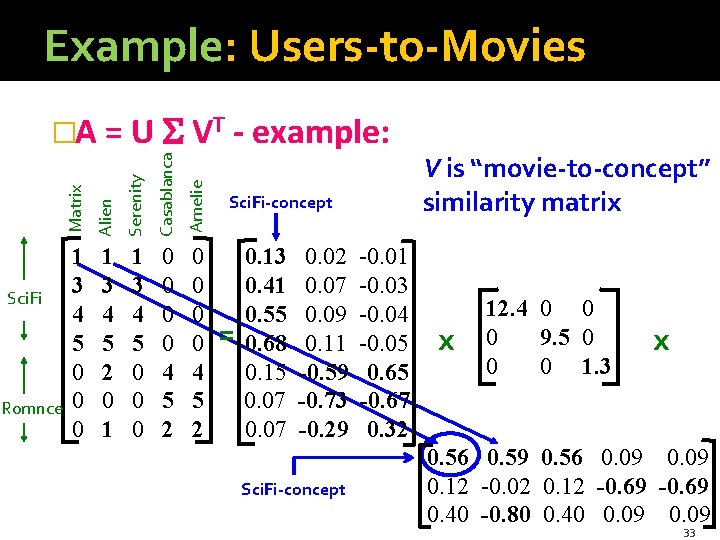
Jure’s Example Decomposition �The following is Example 11. 9 from MMDS. �It modifies the simpler Example 11. 8, where a rank-2 matrix can be decomposed exactly into a 7 -by-2 U and a 5 -by-2 V. 28

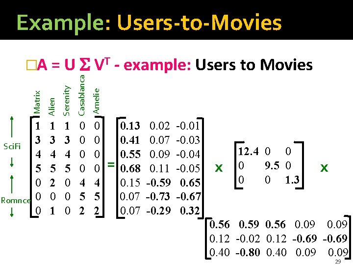
Example: Users-to-Movies Serenity Casablanca Amelie Romnce Alien Sci. Fi Matrix �A = U VT - example: Users to Movies 1 3 4 5 0 0 0 1 3 4 5 2 0 1 1 3 4 5 0 0 0 0 4 5 2 = 0. 13 0. 41 0. 55 0. 68 0. 15 0. 07 0. 02 0. 07 0. 09 0. 11 -0. 59 -0. 73 -0. 29 -0. 01 -0. 03 -0. 04 -0. 05 0. 65 -0. 67 0. 32 x 12. 4 0 0 0 9. 5 0 0 0 1. 3 x 0. 56 0. 59 0. 56 0. 09 0. 12 -0. 02 0. 12 -0. 69 0. 40 -0. 80 0. 40 0. 09 29

Example: Users-to-Movies Serenity Casablanca Amelie Romnce Alien Sci. Fi Matrix �A = U VT - example: Users to Movies 1 3 4 5 0 0 0 1 3 4 5 2 0 1 1 3 4 5 0 0 0 0 4 5 2 Sci. Fi-concept Romance-concept = 0. 13 0. 41 0. 55 0. 68 0. 15 0. 07 0. 02 0. 07 0. 09 0. 11 -0. 59 -0. 73 -0. 29 -0. 01 -0. 03 -0. 04 -0. 05 0. 65 -0. 67 0. 32 x 12. 4 0 0 0 9. 5 0 0 0 1. 3 x 0. 56 0. 59 0. 56 0. 09 0. 12 -0. 02 0. 12 -0. 69 0. 40 -0. 80 0. 40 0. 09 30

Example: Users-to-Movies Serenity Casablanca Amelie Romnce Alien Sci. Fi Matrix �A = U VT - example: 1 3 4 5 0 0 0 1 3 4 5 2 0 1 1 3 4 5 0 0 0 0 4 5 2 Sci. Fi-concept = 0. 13 0. 41 0. 55 0. 68 0. 15 0. 07 0. 02 0. 07 0. 09 0. 11 -0. 59 -0. 73 -0. 29 U is “user-to-concept” similarity matrix Romance-concept -0. 01 -0. 03 -0. 04 -0. 05 0. 65 -0. 67 0. 32 x 12. 4 0 0 0 9. 5 0 0 0 1. 3 x 0. 56 0. 59 0. 56 0. 09 0. 12 -0. 02 0. 12 -0. 69 0. 40 -0. 80 0. 40 0. 09 31

Example: Users-to-Movies Serenity Casablanca Amelie Romnce Alien Sci. Fi Matrix �A = U VT - example: 1 3 4 5 0 0 0 1 3 4 5 2 0 1 1 3 4 5 0 0 0 0 4 5 2 Sci. Fi-concept “strength” of the Sci. Fi-concept = 0. 13 0. 41 0. 55 0. 68 0. 15 0. 07 0. 02 0. 07 0. 09 0. 11 -0. 59 -0. 73 -0. 29 -0. 01 -0. 03 -0. 04 -0. 05 0. 65 -0. 67 0. 32 x 12. 4 0 0 0 9. 5 0 0 0 1. 3 x 0. 56 0. 59 0. 56 0. 09 0. 12 -0. 02 0. 12 -0. 69 0. 40 -0. 80 0. 40 0. 09 32

Example: Users-to-Movies Serenity Casablanca Amelie Romnce Alien Sci. Fi Matrix �A = U VT - example: 1 3 4 5 0 0 0 1 3 4 5 2 0 1 1 3 4 5 0 0 0 0 4 5 2 Sci. Fi-concept = 0. 13 0. 41 0. 55 0. 68 0. 15 0. 07 0. 02 0. 07 0. 09 0. 11 -0. 59 -0. 73 -0. 29 Sci. Fi-concept -0. 01 -0. 03 -0. 04 -0. 05 0. 65 -0. 67 0. 32 V is “movie-to-concept” similarity matrix x 12. 4 0 0 0 9. 5 0 0 0 1. 3 x 0. 56 0. 59 0. 56 0. 09 0. 12 -0. 02 0. 12 -0. 69 0. 40 -0. 80 0. 40 0. 09 33

Lowering the Dimension �Q: How exactly is dimensionality reduction done? �A: Set smallest singular values to zero 1 3 4 5 0 0 0 1 3 4 5 2 0 1 1 3 4 5 0 0 0 0 4 5 2 0. 13 0. 41 0. 55 0. 68 0. 15 0. 07 0. 02 0. 07 0. 09 0. 11 -0. 59 -0. 73 -0. 29 -0. 01 -0. 03 -0. 04 -0. 05 0. 65 -0. 67 0. 32 x 12. 4 0 0 0 9. 5 0 0 0 1. 3 x 0. 56 0. 59 0. 56 0. 09 0. 12 -0. 02 0. 12 -0. 69 0. 40 -0. 80 0. 40 0. 09 34

Lowering the Dimension �Q: How exactly is dimensionality reduction done? �A: Set smallest singular values to zero 1 3 4 5 0 0 0 1 3 4 5 2 0 1 1 3 4 5 0 0 0 0 4 5 2 0. 13 0. 41 0. 55 0. 68 0. 15 0. 07 0. 02 0. 07 0. 09 0. 11 -0. 59 -0. 73 -0. 29 -0. 01 -0. 03 -0. 04 -0. 05 0. 65 -0. 67 0. 32 x 12. 4 0 0 0 9. 5 0 0 0 1. 3 x 0. 56 0. 59 0. 56 0. 09 0. 12 -0. 02 0. 12 -0. 69 0. 40 -0. 80 0. 40 0. 09 35

Lowering the Dimension �Q: How exactly is dimensionality reduction done? �A: Set smallest singular values to zero 1 3 4 5 0 0 0 1 3 4 5 2 0 1 1 3 4 5 0 0 0 0 4 5 2 0. 13 0. 41 0. 55 0. 68 0. 15 0. 07 0. 02 0. 07 0. 09 0. 11 -0. 59 -0. 73 -0. 29 x 12. 4 0 0 9. 5 x 0. 56 0. 59 0. 56 0. 09 0. 12 -0. 02 0. 12 -0. 69 36

Lowering the Dimension �Q: How exactly is dimensionality reduction done? �A: Set smallest singular values to zero 1 3 4 5 0 0 0 1 3 4 5 2 0 1 1 3 4 5 0 0 0 0 4 5 2 0. 92 2. 91 3. 90 4. 82 0. 70 -0. 69 0. 32 0. 95 3. 01 4. 04 5. 00 0. 53 1. 34 0. 23 0. 92 2. 91 3. 90 4. 82 0. 70 -0. 69 0. 32 0. 01 -0. 01 0. 03 4. 11 4. 78 2. 01 37

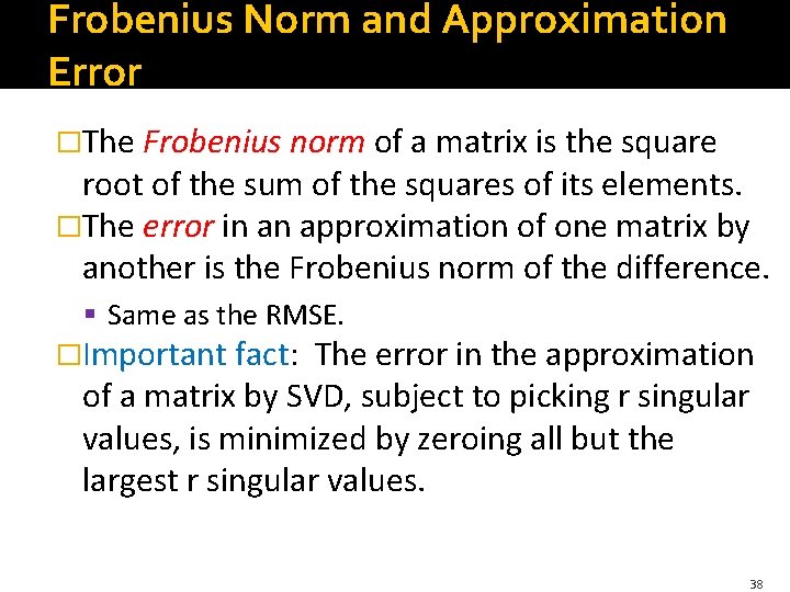
Frobenius Norm and Approximation Error �The Frobenius norm of a matrix is the square root of the sum of the squares of its elements. �The error in an approximation of one matrix by another is the Frobenius norm of the difference. § Same as the RMSE. �Important fact: The error in the approximation of a matrix by SVD, subject to picking r singular values, is minimized by zeroing all but the largest r singular values. 38

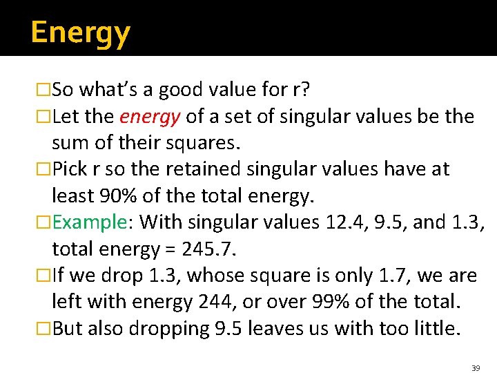
Energy �So what’s a good value for r? �Let the energy of a set of singular values be the sum of their squares. �Pick r so the retained singular values have at least 90% of the total energy. �Example: With singular values 12. 4, 9. 5, and 1. 3, total energy = 245. 7. �If we drop 1. 3, whose square is only 1. 7, we are left with energy 244, or over 99% of the total. �But also dropping 9. 5 leaves us with too little. 39

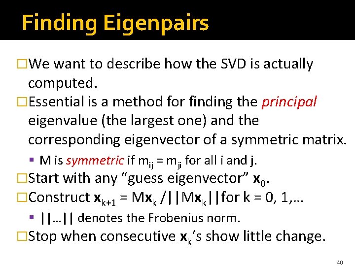
Finding Eigenpairs �We want to describe how the SVD is actually computed. �Essential is a method for finding the principal eigenvalue (the largest one) and the corresponding eigenvector of a symmetric matrix. § M is symmetric if mij = mji for all i and j. �Start with any “guess eigenvector” x 0. �Construct xk+1 = Mxk /||Mxk||for k = 0, 1, … § ||…|| denotes the Frobenius norm. �Stop when consecutive xk‘s show little change. 40

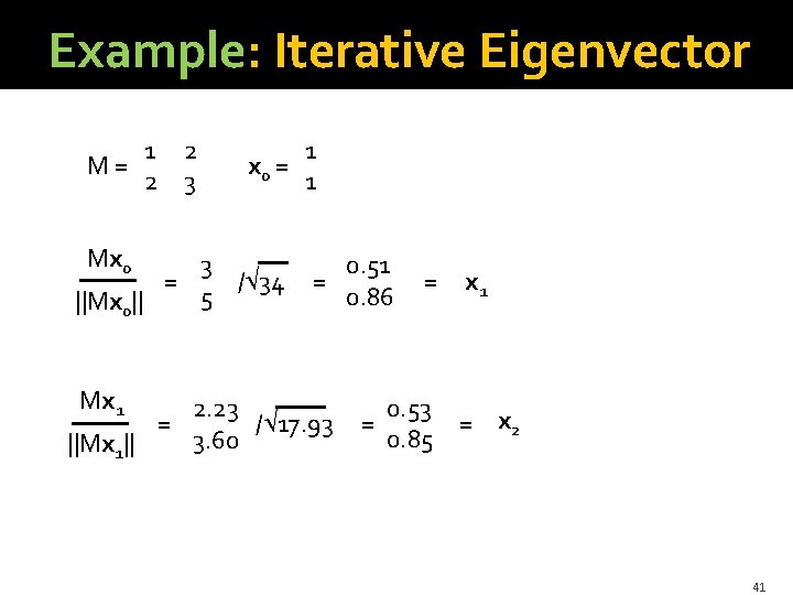
Example: Iterative Eigenvector 1 2 M= 2 3 Mx 0 ||Mx 0|| Mx 1 = 1 x 0 = 1 3 / 34 5 = 2. 23 = / 17. 93 3. 60 ||Mx 1|| 0. 51 0. 86 = x 1 0. 53 = = x 2 0. 85 41

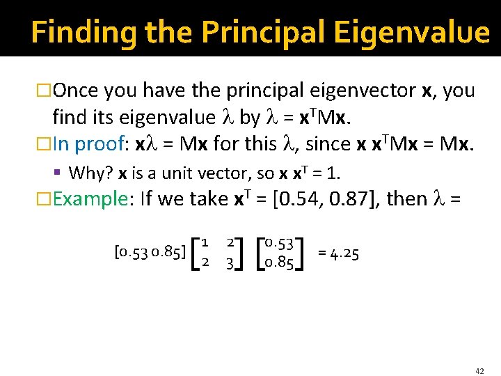
Finding the Principal Eigenvalue �Once you have the principal eigenvector x, you find its eigenvalue by = x. TMx. �In proof: x = Mx for this , since x x. TMx = Mx. § Why? x is a unit vector, so x x. T = 1. �Example: If we take x. T = [0. 54, 0. 87], then = [0. 53 0. 85] [ ][ ] 1 2 2 3 0. 53 0. 85 = 4. 25 42

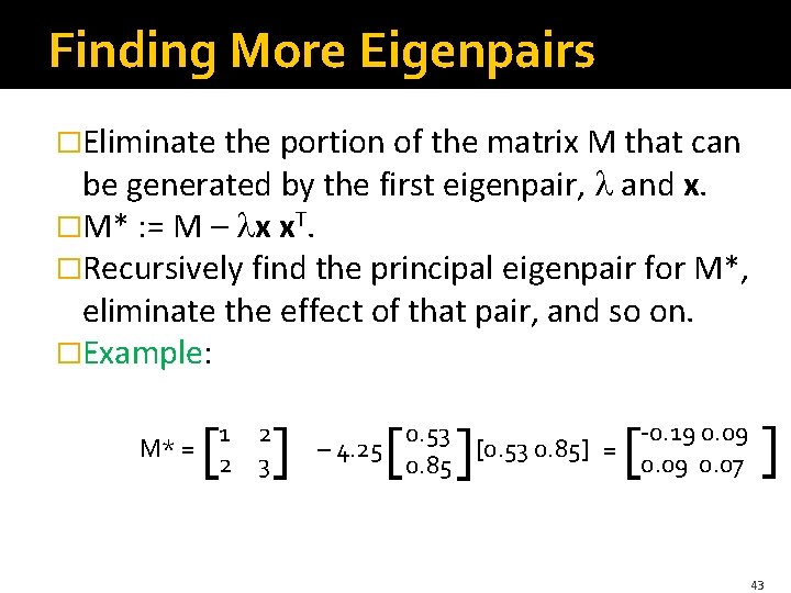
Finding More Eigenpairs �Eliminate the portion of the matrix M that can be generated by the first eigenpair, and x. �M* : = M – x x. T. �Recursively find the principal eigenpair for M*, eliminate the effect of that pair, and so on. �Example: [ ] 1 2 M* = 2 3 [ ] [ -0. 19 0. 09 0. 53 [0. 53 0. 85] = – 4. 25 0. 09 0. 07 0. 85 ] 43

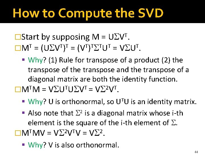
How to Compute the SVD �Start by supposing M = U VT. �MT = (U VT)T = (VT)T TUT = V UT. § Why? (1) Rule for transpose of a product (2) the transpose of the transpose and the transpose of a diagonal matrix are both the identity function. �MTM = V UTU VT = V 2 VT. § Why? U is orthonormal, so UTU is an identity matrix. § Also note that 2 is a diagonal matrix whose i-th element is the square of the i-th element of . �MTMV = V 2 VTV = V 2. § Why? V is also orthonormal. 44

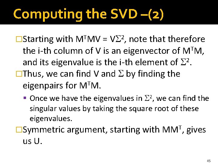
Computing the SVD –(2) �Starting with MTMV = V 2, note that therefore the i-th column of V is an eigenvector of MTM, and its eigenvalue is the i-th element of 2. �Thus, we can find V and by finding the eigenpairs for MTM. § Once we have the eigenvalues in 2, we can find the singular values by taking the square root of these eigenvalues. �Symmetric argument, starting with MMT, gives us U. 45

CUR Decomposition The Sparsity Issue Picking Random Rows and Columns

Sparsity �It is common for the matrix M that we wish to decompose to be very sparse. �But U and V from a UV or SVD decomposition will not be sparse even so. �CUR decomposition solves this problem by using only (randomly chosen) rows and columns of M. 47

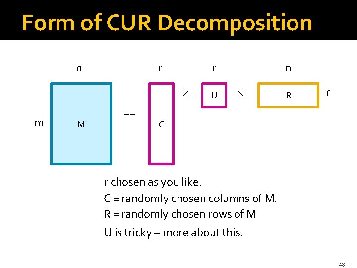
Form of CUR Decomposition n r m M ~~ n r U R r C r chosen as you like. C = randomly chosen columns of M. R = randomly chosen rows of M U is tricky – more about this. 48

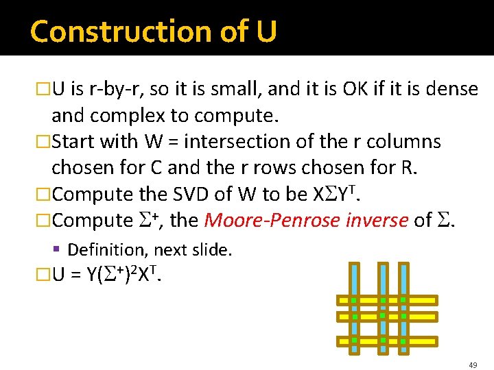
Construction of U �U is r-by-r, so it is small, and it is OK if it is dense and complex to compute. �Start with W = intersection of the r columns chosen for C and the r rows chosen for R. �Compute the SVD of W to be X YT. �Compute +, the Moore-Penrose inverse of . § Definition, next slide. �U = Y( +)2 XT. 49

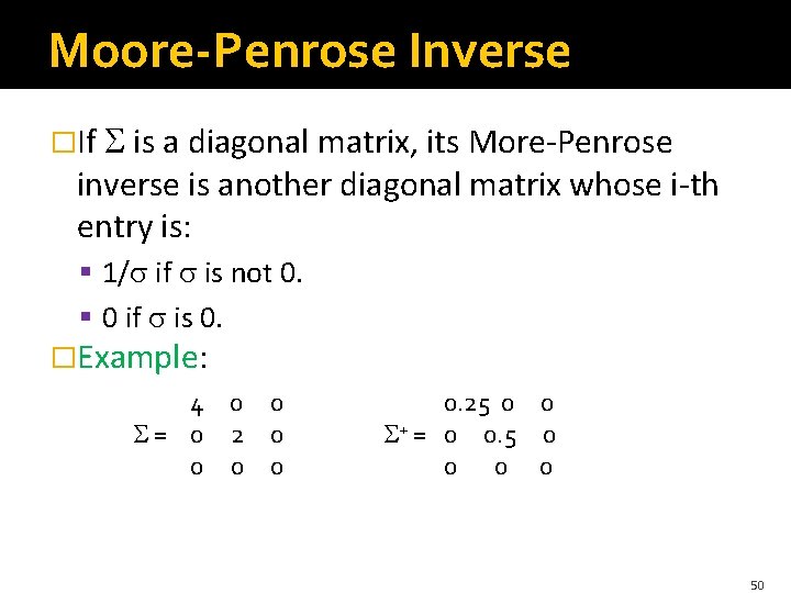
Moore-Penrose Inverse �If is a diagonal matrix, its More-Penrose inverse is another diagonal matrix whose i-th entry is: § 1/ if is not 0. § 0 if is 0. �Example: 4 0 0 = 0 2 0 0 0. 25 0 0 + = 0 0. 5 0 0 50

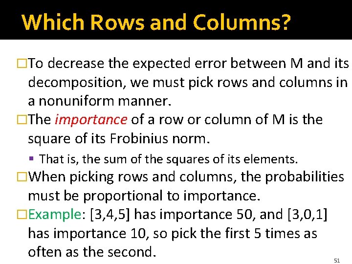
Which Rows and Columns? �To decrease the expected error between M and its decomposition, we must pick rows and columns in a nonuniform manner. �The importance of a row or column of M is the square of its Frobinius norm. § That is, the sum of the squares of its elements. �When picking rows and columns, the probabilities must be proportional to importance. �Example: [3, 4, 5] has importance 50, and [3, 0, 1] has importance 10, so pick the first 5 times as often as the second. 51