Introduction to Numerical Solutions of Ordinary Differential Equations

Introduction to Numerical Solutions of Ordinary Differential Equations Larry Caretto Mechanical Engineering 501 AB Seminar in Engineering Analysis October 29, 2003

Outline • Review last class and homework • Midterm Exam November 4 covers material up to and including last week’s lecture • Overivew of numerical solutions – Initial value problems in first-order equations – Systems of first order equations and initial value problems in higher order equations – Boundary value problems – Stiff systems and eigenvalues 2

Review Last Class • Systems of equations – Combine to higher order equation – Matrix approaches – Reduction of order • Laplace transforms for ODEs – Transform ODE from y(t) to Y(s) – Solve for Y(s) – Rearrange solution – Transform back to y(t) 3

Simultaneous Solution • Differentiate first (y 1) equation to obtain derivative(s) of y 2 that are present in second equation • Solve first equation for y 2 • Substitute equations for y 2 and its derivatives into the result of the first step • Result is a higher order equation that can be solved (if possible) by usual methods 4

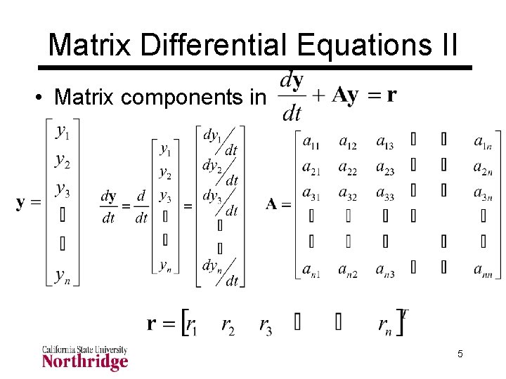
Matrix Differential Equations II • Matrix components in 5

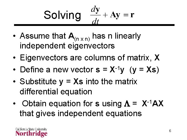
Solving • Assume that A(n x n) has n linearly independent eigenvectors • Eigenvectors are columns of matrix, X • Define a new vector s = X-1 y (y = Xs) • Substitute y = Xs into the matrix differential equation • Obtain equation for s using L = X-1 AX that gives independent equations 6

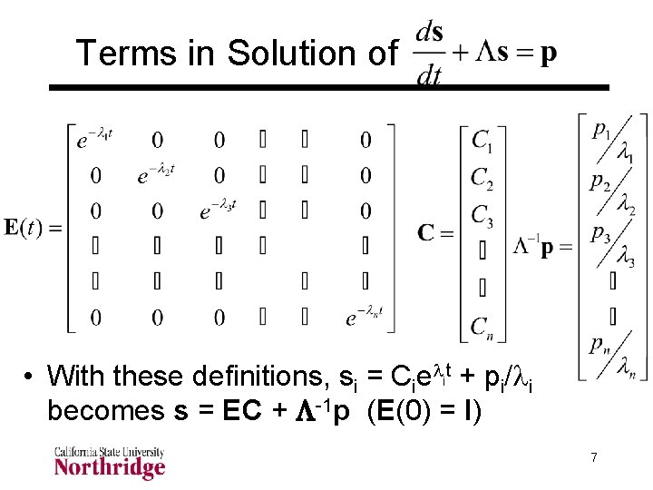
Terms in Solution of • With these definitions, si = Cielit + pi/li becomes s = EC + L-1 p (E(0) = I) 7

Apply Initial Conditions on y(0) • Get y = Xs = XEC + XL-1 p • At t = 0, E = I, and y = y 0 = initial y components, giving y 0 = XIC + XL-1 p • Premultiply by X-1 to obtain X-1 y 0 = X 1 XC + X-1 XL-1 p = C + L-1 p • Constant vector, C = X-1 y 0 - L-1 p • Result: y = XE [X-1 y 0 - L-1 p] + XL-1 p • Homogenous(p = 0): y = XEX-1 y 0 8

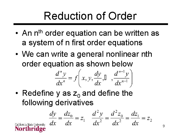
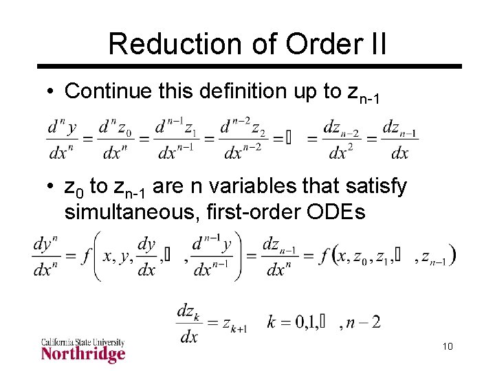
Reduction of Order • An nth order equation can be written as a system of n first order equations • We can write a general nonlinear nth order equation as shown below • Redefine y as z 0 and define the following derivatives 9

Reduction of Order II • Continue this definition up to zn-1 • z 0 to zn-1 are n variables that satisfy simultaneous, first-order ODEs 10

Reduction of Order III • The main application of reduction of order is to numerical methods • Numerical solutions of ODEs develop methods to solve a system of first order equations • Higher order equations are solved by converting them to a system of first order equations 11

Simple Laplace Transforms f(t) F(s) f(t) ctn cn!/sn+1 ceatsin wt ctx c. G(x+1)/sx+1 ceat c/(s – a) csin wt cw/(s 2 + w 2) ccos wt cs/(s 2 + w 2) Additional transforms in cw/(s 2 - w 2) Table 5. 9, pp 297 -299 of Kreyszig cs/(s 2 - w 2) csinh wt ccosh wt F(s) ceatcos wt 12

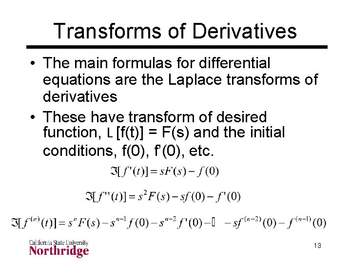
Transforms of Derivatives • The main formulas for differential equations are the Laplace transforms of derivatives • These have transform of desired function, L [f(t)] = F(s) and the initial conditions, f(0), f’(0), etc. 13

Solving Differential Equations • Transform all terms in the differential equation to get an algebraic equation – For a differential equation in y(t) we get the transforms Y(s) = L [y(t)] – Similar notation for other transformed functions in the equation R(s) = L [r(t)] • Solve the algebraic equation for Y(s) • Obtain the inverse transform for Y(s) from tables to get y(t) 14

Partial Fractions • Method to convert fraction with several factors in denominator into sum of individual factors (in denominator) • Necessary to modify complicated solution for Y(s) into simpler functions whose transforms are known • Special rules for repeated factors and for complex conjugates 15

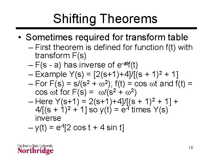
Shifting Theorems • Sometimes required for transform table – First theorem is defined for function f(t) with transform F(s) – F(s - a) has inverse of e-atf(t) – Example Y(s) = [2(s+1)+4]/[(s + 1)2 + 1] – For F(s) = s/(s 2 + w 2); f(t) = cos wt and f(t) = cos wt for F(s) = w/(s 2 + w 2) – Here Y(s+1) = 2(s+1)+4]/[(s + 1)2 + 1] + 4/[(s + 1)2 + 1] so y(t) = e-t times Y(s) inverse – y(t) = e-t[2 cos t + 4 sin t] 16

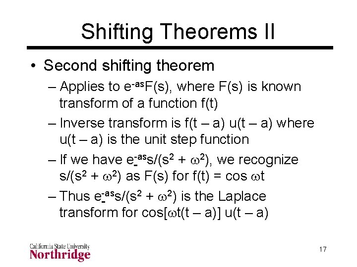
Shifting Theorems II • Second shifting theorem – Applies to e-as. F(s), where F(s) is known transform of a function f(t) – Inverse transform is f(t – a) u(t – a) where u(t – a) is the unit step function – If we have e-ass/(s 2 + w 2), we recognize s/(s 2 + w 2) as F(s) for f(t) = cos wt – Thus e-ass/(s 2 + w 2) is the Laplace transform for cos[wt(t – a)] u(t – a) 17

Numerical Analysis Problems • Numerical solution of algebraic equations and eigenvalue problems • Solution of one or more nonlinear algebraic equations f(x) = 0 • Linear and nonlinear optimization • Constructing interpolating polynomials • Numerical quadrature • Numerical differentiation • Numerical differential equations 18

Interpolation • Start with N data pairs xi, yi • Find a function (polynomial) that can be used for interpolation • Basic rule: the interpolation polynomial must fit all points exactly • Denote the polynomial as p(x) • The basic rule is that p(xi) = yi • Many different forms 19

Newton Polynomials • p(x) = a 0 + a 1(x – x 0) + a 2(x – x 0)(x – x 1) + a 3(x – x 0)(x – x 1)(x – x 2) + … + an-1(x – x 0)(x – x 1)(x – x 2) … (x – xn-2) • Terms with factors of x – xi are zero when x = xi – Use this and rule that p(xi) = yi to find ai • a 0 = y 0, a 1 = (y 1 – y 0) / (x 1 – x 0) • y 2 = a 0 + a 1(x 2 – x 0) + a 2(x 2 – x 0)(x 2 – x 1) – Solve for a 2 using results for a 0 and a 1 20

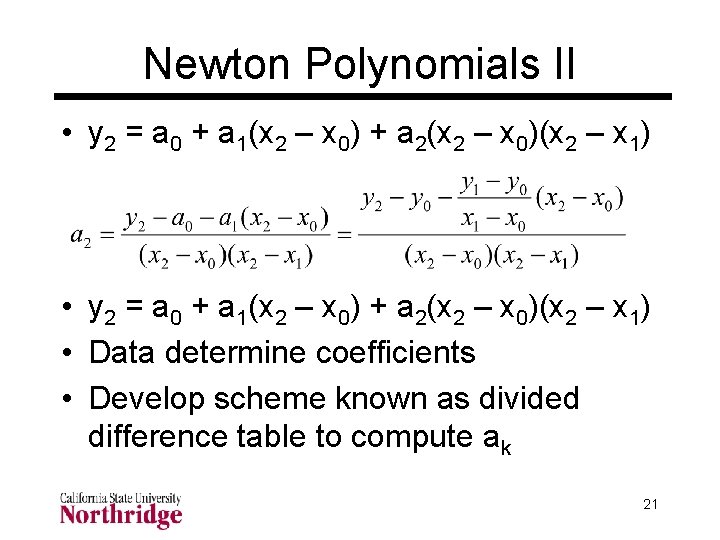
Newton Polynomials II • y 2 = a 0 + a 1(x 2 – x 0) + a 2(x 2 – x 0)(x 2 – x 1) • Data determine coefficients • Develop scheme known as divided difference table to compute ak 21

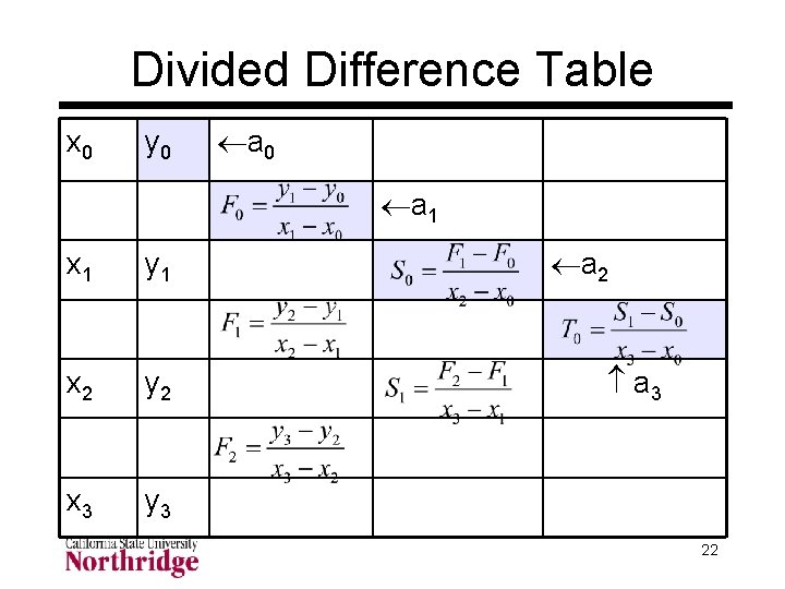
Divided Difference Table x 0 y 0 a 0 a 1 x 1 y 1 x 2 y 2 x 3 y 3 a 2 a 3 22

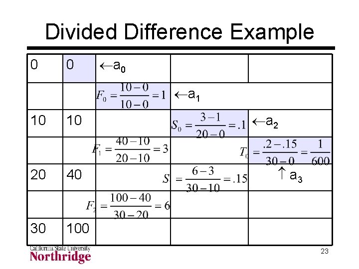
Divided Difference Example 0 0 a 0 a 1 10 10 20 40 30 100 a 2 a 3 23

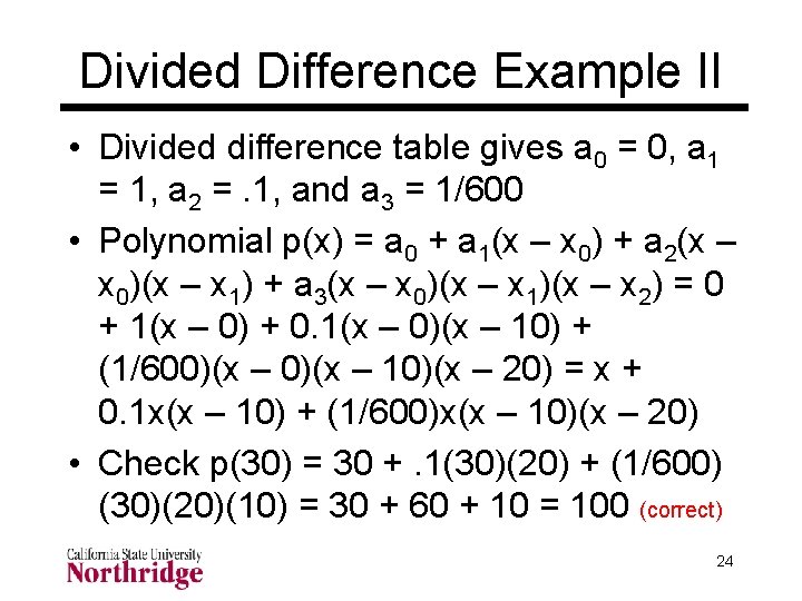
Divided Difference Example II • Divided difference table gives a 0 = 0, a 1 = 1, a 2 =. 1, and a 3 = 1/600 • Polynomial p(x) = a 0 + a 1(x – x 0) + a 2(x – x 0)(x – x 1) + a 3(x – x 0)(x – x 1)(x – x 2) = 0 + 1(x – 0) + 0. 1(x – 0)(x – 10) + (1/600)(x – 10)(x – 20) = x + 0. 1 x(x – 10) + (1/600)x(x – 10)(x – 20) • Check p(30) = 30 +. 1(30)(20) + (1/600) (30)(20)(10) = 30 + 60 + 10 = 100 (correct) 24

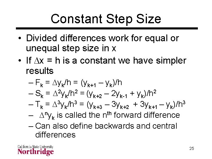
Constant Step Size • Divided differences work for equal or unequal step size in x • If Dx = h is a constant we have simpler results – Fk = Dyk/h = (yk+1 – yk)/h – Sk = D 2 yk/h 2 = (yk+2 – 2 yk-1 + yk)/h 2 – Tk = D 3 yk/h 3 = (yk+3 – 3 yk+2 + 3 yk+1 – yk)/h 3 – Dnyk is called the nth forward difference – Can also define backwards and central differences 25

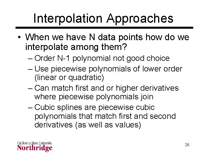
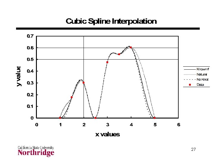
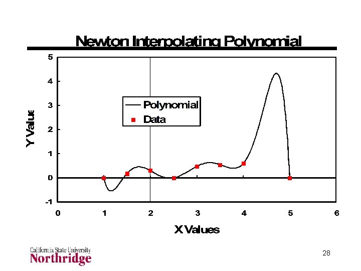
Interpolation Approaches • When we have N data points how do we interpolate among them? – Order N-1 polynomial not good choice – Use piecewise polynomials of lower order (linear or quadratic) – Can match first and or higher derivatives where piecewise polynomials join – Cubic splines are piecewise cubic polynomials that match first and second derivatives (as well as values) 26

27

28

Polynomial Applications • Data interpolation • Approximation functions in numerical quadrature and solution of ODEs • Basis functions for finite element methods • Can obtain equations for numerical differentiation • Statistical curve fitting (not discussed here) usually used in practice 29

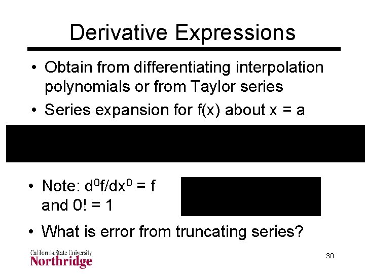
Derivative Expressions • Obtain from differentiating interpolation polynomials or from Taylor series • Series expansion for f(x) about x = a • Note: d 0 f/dx 0 = f and 0! = 1 • What is error from truncating series? 30

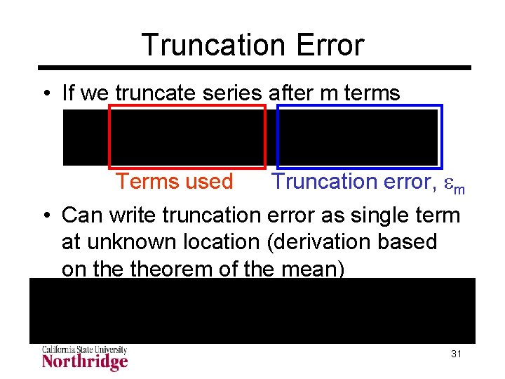
Truncation Error • If we truncate series after m terms Terms used Truncation error, em • Can write truncation error as single term at unknown location (derivation based on theorem of the mean) 31

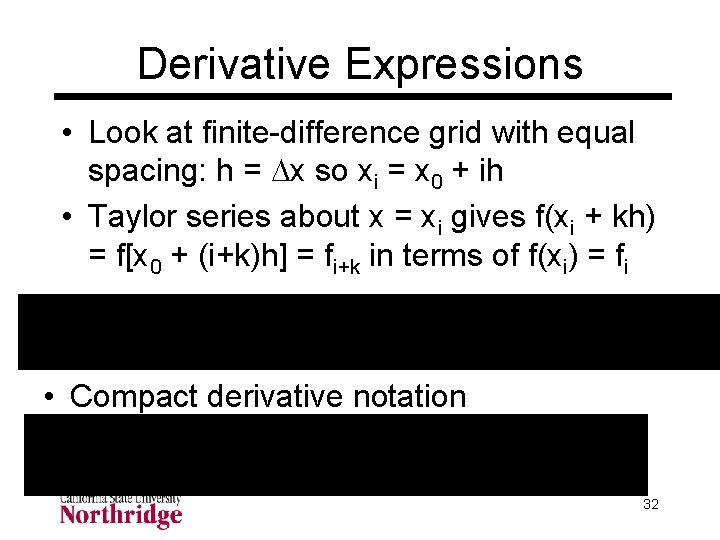
Derivative Expressions • Look at finite-difference grid with equal spacing: h = Dx so xi = x 0 + ih • Taylor series about x = xi gives f(xi + kh) = f[x 0 + (i+k)h] = fi+k in terms of f(xi) = fi • Compact derivative notation 32

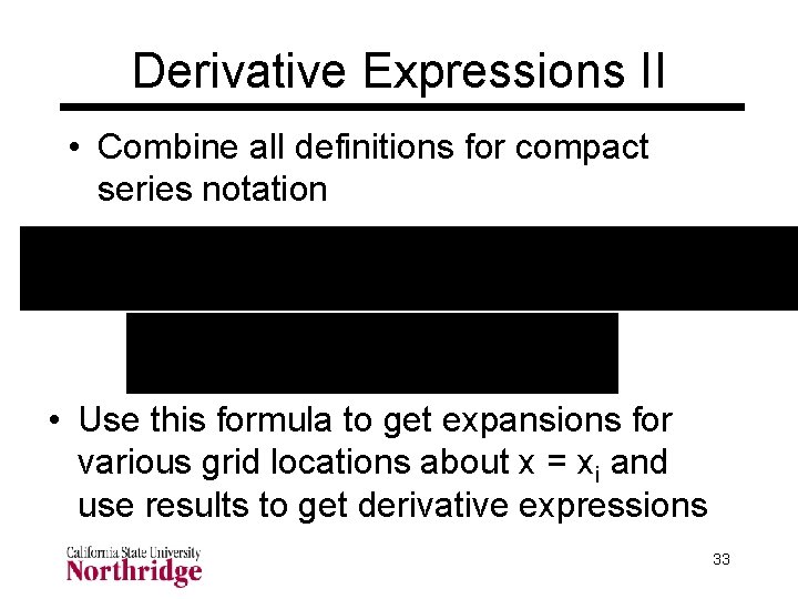
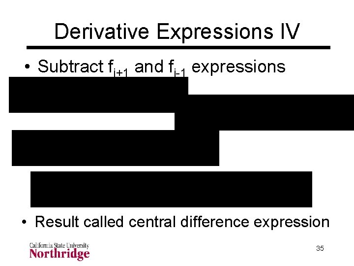
Derivative Expressions II • Combine all definitions for compact series notation • Use this formula to get expansions for various grid locations about x = xi and use results to get derivative expressions 33

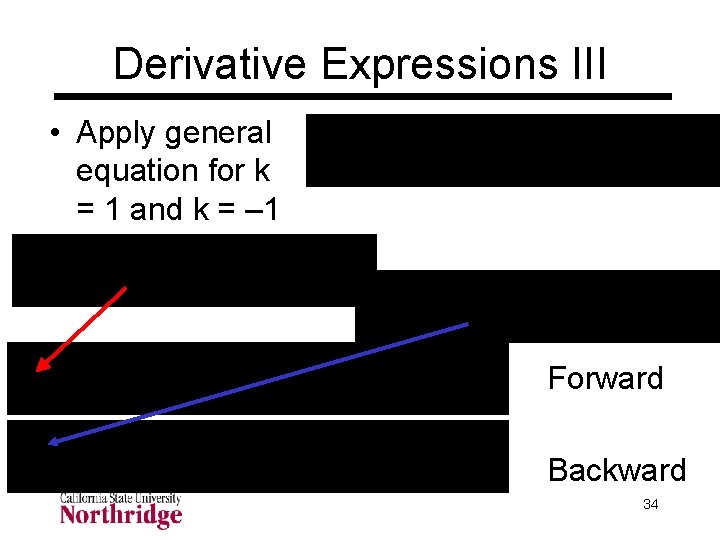
Derivative Expressions III • Apply general equation for k = 1 and k = – 1 Forward Backward 34

Derivative Expressions IV • Subtract fi+1 and fi-1 expressions • Result called central difference expression 35

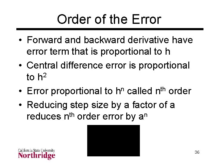
Order of the Error • Forward and backward derivative have error term that is proportional to h • Central difference error is proportional to h 2 • Error proportional to hn called nth order • Reducing step size by a factor of a reduces nth order error by an 36

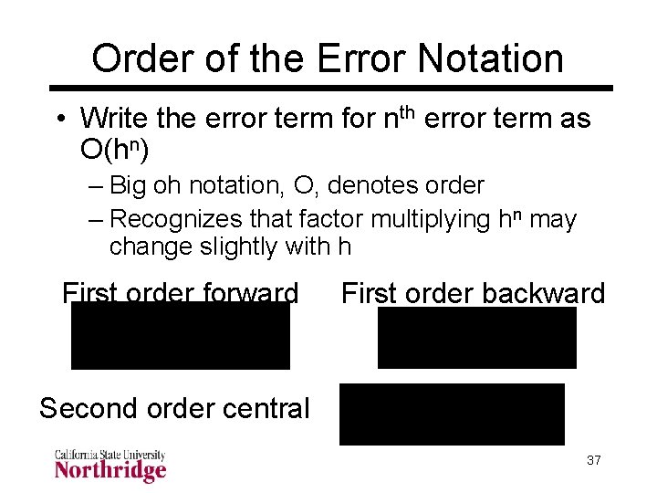
Order of the Error Notation • Write the error term for nth error term as O(hn) – Big oh notation, O, denotes order – Recognizes that factor multiplying hn may change slightly with h First order forward First order backward Second order central 37

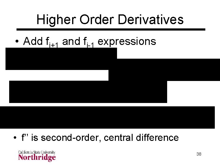
Higher Order Derivatives • Add fi+1 and fi-1 expressions • f’’ is second-order, central difference 38

Higher Order Directional • We can get higher order derivative expressions at the expense of more computations • Get second order forward and backward derivative expressions from fi+2 and fi-2, respectively • Combine with previous expressions for fi+1 and fi-1 to eliminate first order error term 39

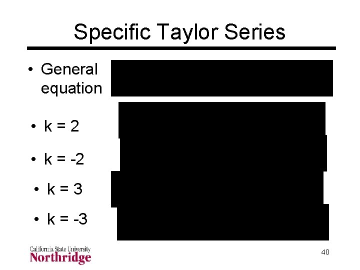
Specific Taylor Series • General equation • k=2 • k = -2 • k=3 • k = -3 40

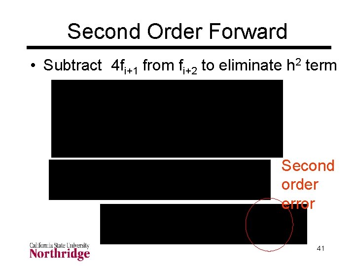
Second Order Forward • Subtract 4 fi+1 from fi+2 to eliminate h 2 term Second order error 41

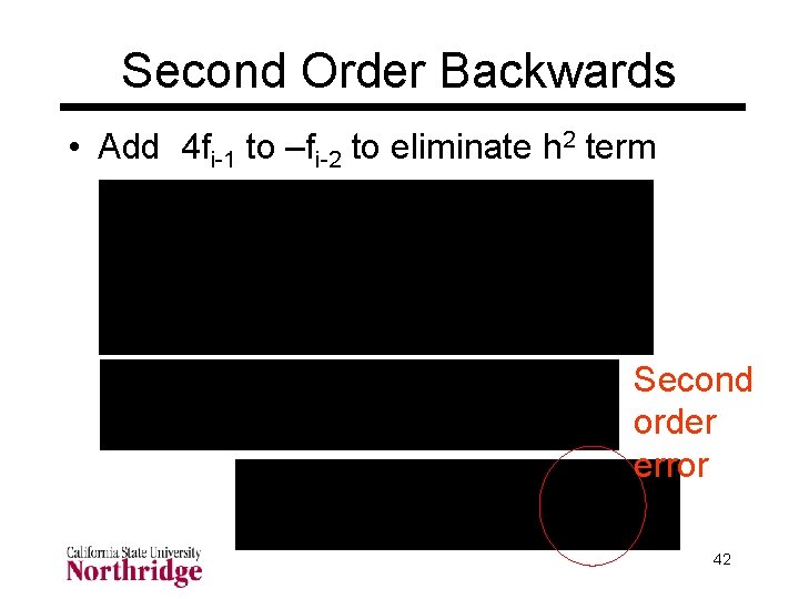
Second Order Backwards • Add 4 fi-1 to –fi-2 to eliminate h 2 term Second order error 42

Other Derivative Expressions • Can continue in this fashion – Write Taylor series for fi+1, fi-1, fi+2, fi-2, fi+3, fi 3, etc. – Create linear combinations with factors that eliminate desired terms – Eliminate fi term to obtain central difference – Keep only terms in fk with k i for forward difference expressions – See results on page 271 of Hoffman 43

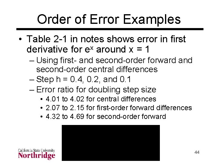
Order of Error Examples • Table 2 -1 in notes shows error in first derivative for ex around x = 1 – Using first- and second-order forward and second-order central differences – Step h = 0. 4, 0. 2, and 0. 1 – Error ratio for doubling step size • 4. 01 to 4. 02 for central differences • 2. 07 to 2. 15 for first-order forward differences • 4. 32 to 4. 69 for second-order forward 44

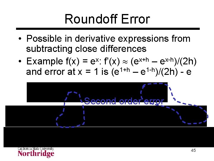
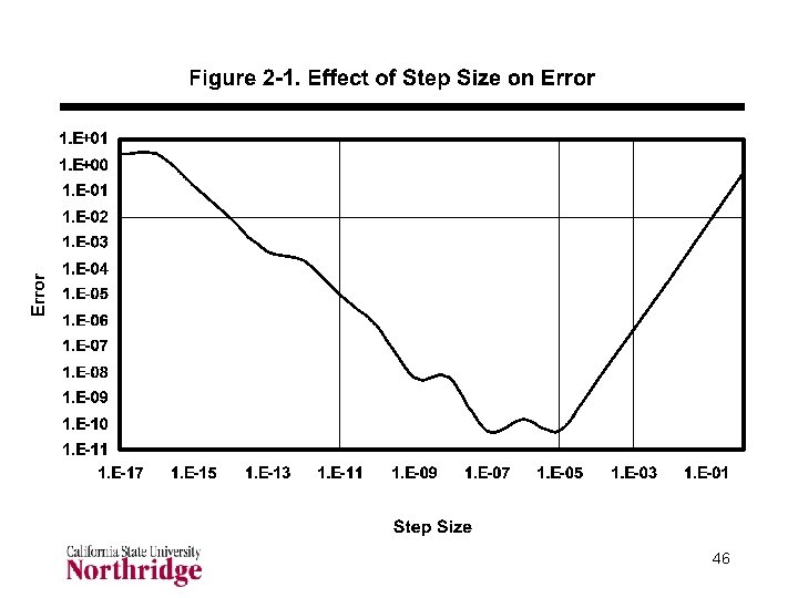
Roundoff Error • Possible in derivative expressions from subtracting close differences • Example f(x) = ex: f’(x) (ex+h – ex-h)/(2 h) and error at x = 1 is (e 1+h – e 1 -h)/(2 h) - e Second order error 45

46

Numerical ODE Solutions • The initial value problem • Euler method as a prototype for the general algorithm • Local and global errors • More accurate methods • Step-size control for error control • Applications to systems of equations • Higher-order equations 47

The Initial Value Problem • dy/dx = f(x, y) (known) with y(x 0) = y 0 • Basic numerical approach – Use a finite difference grid: xi+1 – xi = h – Replace derivative by finite-difference approximation: dy/dx (yi+1 – yi) / (xi+1 – xi) = (yi+1 – yi) / h – Derive a formula to compute favg the average value of f(x, y) between xi and xi+1 – Replace dy/dx = f(x, y) by (yi+1 – yi) / h = favg – Repeatedly compute yi+1 = yi + h favg 48

Notation • xi is the value of the independent variable at point i on the grid – Determined from the user-selected value of step size (or the series of hi values) – Can always specify exactly the independent variable’s value, xi • yi is the value of the numerical solution at the point where x = xi • fi is derivative value found from xi and the numerical value, yi. I. e. , fi = f(xi, yi). 49

More Notation • y(xi) is the exact value of y at x = xi – Usually not known but notation is used in error analysis of algorithms • f(xi, y(xi)) is the exact value of the derivative at x = xi • e 1 = y(x 1) – y 1 is the local truncation error – This is error for one step of algorithm starting from known initial condition 50

Local versus Global Error • At the initial condition we know the solution, y, exactly • First step introduces some error • Remaining steps have single step error plus previous accumulated error • Ej = y(xj) – yj is global truncation error – Difference between numerical and exact solution after several steps – This is the error we want to control 51

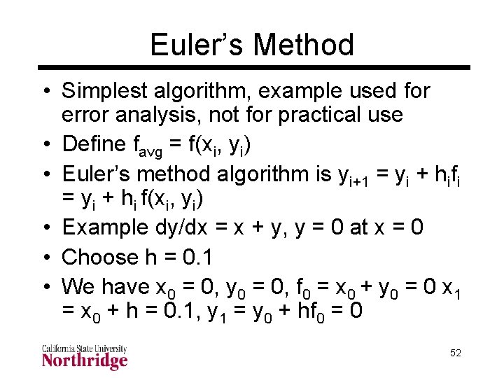
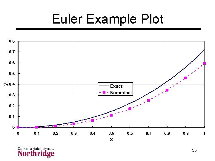
Euler’s Method • Simplest algorithm, example used for error analysis, not for practical use • Define favg = f(xi, yi) • Euler’s method algorithm is yi+1 = yi + hifi = yi + hi f(xi, yi) • Example dy/dx = x + y, y = 0 at x = 0 • Choose h = 0. 1 • We have x 0 = 0, y 0 = 0, f 0 = x 0 + y 0 = 0 x 1 = x 0 + h = 0. 1, y 1 = y 0 + hf 0 = 0 52

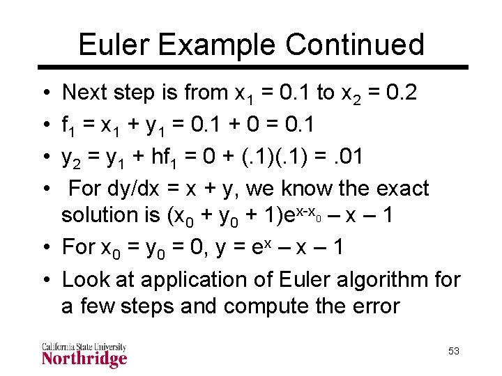
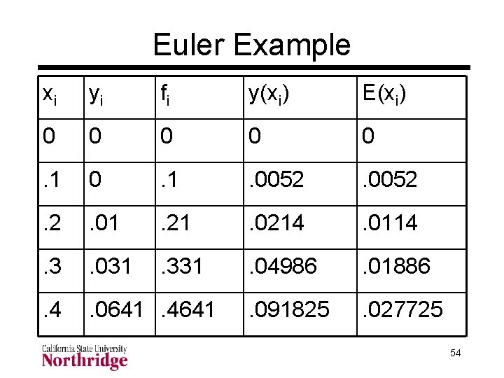
Euler Example Continued • • Next step is from x 1 = 0. 1 to x 2 = 0. 2 f 1 = x 1 + y 1 = 0. 1 + 0 = 0. 1 y 2 = y 1 + hf 1 = 0 + (. 1) =. 01 For dy/dx = x + y, we know the exact solution is (x 0 + y 0 + 1)ex-x 0 – x – 1 • For x 0 = y 0 = 0, y = ex – 1 • Look at application of Euler algorithm for a few steps and compute the error 53

Euler Example xi yi fi y(xi) E(xi) 0 0 0 . 1 . 0052 . 2 . 01 . 21 . 0214 . 0114 . 3 . 031 . 331 . 04986 . 01886 . 4 . 0641. 4641 . 091825 . 027725 54

Euler Example Plot 55

Error Propagation • Behavior of Euler algorithm is typical of all algorithms for numerical solutions • Error grows at each step • We usually do not know this global error, but we would like to control it • Look at local error for Euler algorithm • Then discuss general relationship between local and global error 56

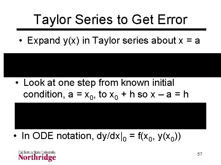
Taylor Series to Get Error • Expand y(x) in Taylor series about x = a • Look at one step from known initial condition, a = x 0, to x 0 + h so x – a = h • In ODE notation, dy/dx|0 = f(x 0, y(x 0)) 57

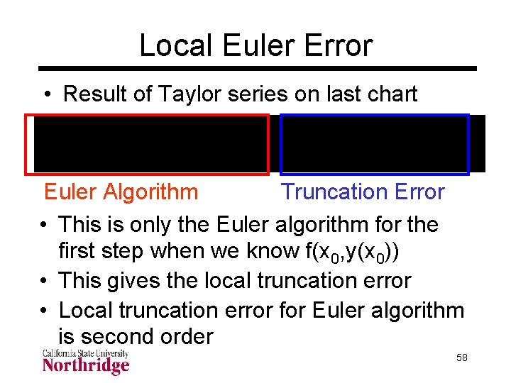
Local Euler Error • Result of Taylor series on last chart Euler Algorithm Truncation Error • This is only the Euler algorithm for the first step when we know f(x 0, y(x 0)) • This gives the local truncation error • Local truncation error for Euler algorithm is second order 58

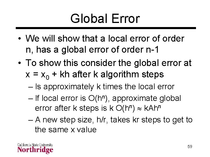
Global Error • We will show that a local error of order n, has a global error of order n-1 • To show this consider the global error at x = x 0 + kh after k algorithm steps – Is approximately k times the local error – If local error is O(hn), approximate global error after k steps is k O(hn) k. Ahn – A new step size, h/r, takes kr steps to get to the same x value 59

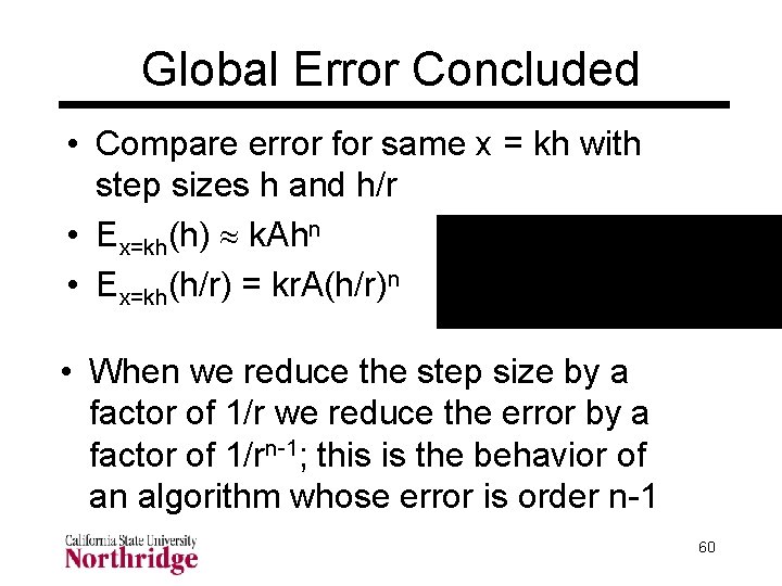
Global Error Concluded • Compare error for same x = kh with step sizes h and h/r • Ex=kh(h) k. Ahn • Ex=kh(h/r) = kr. A(h/r)n • When we reduce the step size by a factor of 1/r we reduce the error by a factor of 1/rn-1; this is the behavior of an algorithm whose error is order n-1 60

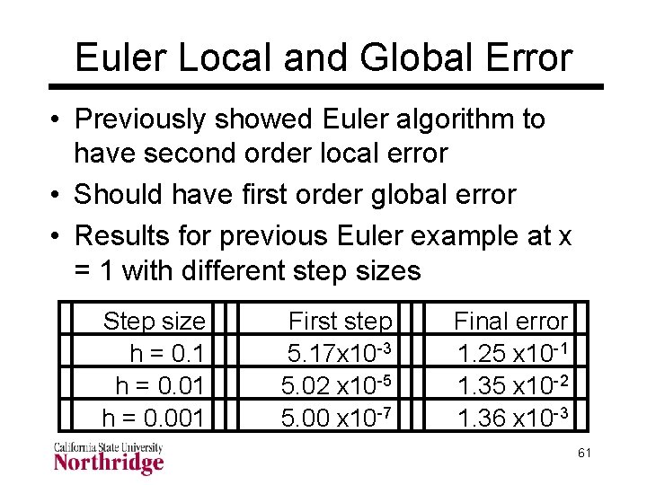
Euler Local and Global Error • Previously showed Euler algorithm to have second order local error • Should have first order global error • Results for previous Euler example at x = 1 with different step sizes Step size h = 0. 1 h = 0. 001 First step 5. 17 x 10 -3 5. 02 x 10 -5 5. 00 x 10 -7 Final error 1. 25 x 10 -1 1. 35 x 10 -2 1. 36 x 10 -3 61

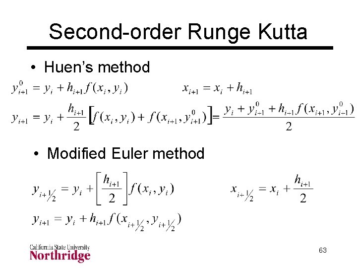
Better Algorithms • Seek high accuracy with low computational work • Could improve Euler accuracy by cutting step size, but this is not efficient • Use other algorithms that have higher order errors • Runge-Kutta methods typically used – This is a class of methods that use several function evaluation methods per step 62

Second-order Runge Kutta • Huen’s method • Modified Euler method 63

Fourth-order Runge Kutta • Uses four derivative evaluations per step 64

Comparison of Methods • Look at Euler, Heun, Modified Euler and fourth-order Runge-Kutta • Solve dy/dx = e-y-x with y(0) = 1 • Compare numerical values to exact solution y = ln( ey 0 + e-x 0 – e-x) • Look at errors in the methods at x = 1 as a function of step size • Compare error propagation (increase in error as x increases) 65

66

67

Some Basic Concepts • A numerical method is convergent with the solution of the ODE if the numerical solution approaches the actual solution as h 0 (with increase in numerical precision at smaller h) – Mainly a theoretical concept; algorithms in use are convergent • Stability refers to the ability of a numerical algorithm to damp any errors introduced during the solution 68

More on Stability • Finite difference equations in numerical algorithms, when iterated, may be numerically increase without bound • Stability usually is obtained by keeping step size h small, sometimes smaller than the h required for accuracy • For most ODEs stability is not a problem, but it is for stiff systems of ODEs and for partial differential equations 69

70

71

Error Control • How do we choose h? • Want to obtain a result with some desired small global error • Can just repeat calculations with smaller h until two results are sufficiently close • Can use algorithms that estimate error and adjust step size during the calculation based on the error 72

Runge-Kutta-Fehlberg • Uses two equations to compute yn+1, one has O(h 5), the other O(h 6) error • Requires six derivative evaluations per step (same evaluations used for both equations) • The error estimate can be used for step size control based on an overall 5 th order error • Cask-Karp version different coefficients 73

Runge-Kutta-Fehlberg II • • See page 377 in Hoffman for algorithm Typical formula components below yn+1= yn + (16 k 1/135 + 6656 k 2/12825 … k 3 = hf(xn + 3 h/8, yn + 3 k 1/32 + 9 k 2/32) Error = k 1/360 - 128 k 3/4275 … hnew = hold|EDesired/Error|1/5 EDesired is set by user RKF 45 code by Watts and Shampine 74

Other Error Controls • Do fourth-order Runge-Kutta two times, with step sizes different by a factor of two and compare results • Runge-Kutta-Verner is similar to Runge. Kutta-Fehlberg, but uses higher order expressions 75

Systems of Equations • Any problem with one or more ODEs of any order can be reduced to a system for first order ODEs • Last week we reduced a system of two second order equations to a system of four first order equations • In this process the sum of the orders is constant • Example from last week 76

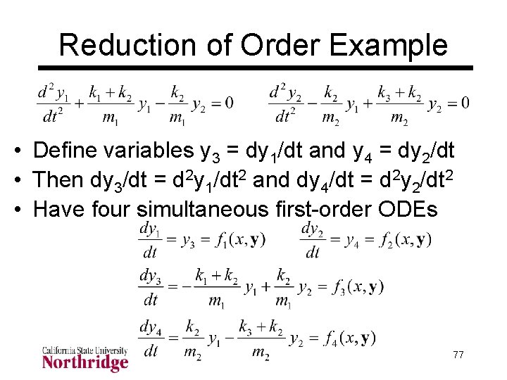
Reduction of Order Example • Define variables y 3 = dy 1/dt and y 4 = dy 2/dt • Then dy 3/dt = d 2 y 1/dt 2 and dy 4/dt = d 2 y 2/dt 2 • Have four simultaneous first-order ODEs 77

Solving Simultaneous ODEs • Apply same algorithms used for single ODEs – Must apply each step and substep to all equations in system – Key is consistent determination of fi(x, y) – All yi values in y must be available at the same x point when computing the fi – E. g. , in Runge-Kutta we must evaluate k 1 for all equations before finding k 2 78

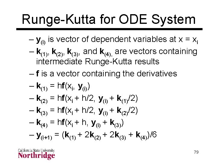
Runge-Kutta for ODE System – y(i) is vector of dependent variables at x = xi – k(1), k(2), k(3), and k(4), are vectors containing intermediate Runge-Kutta results – f is a vector containing the derivatives – k(1) = hf(xi, y(i)) – k(2) = hf(xi + h/2, y(i) + k(1)/2) – k(3) = hf(xi + h/2, y(i) + k(2)/2) – k(4) = hf(xi + h, y(i) + k(3)) – y(i+1) = (k(1) + 2 k(2) + 2 k(3) + k(4))/6 79

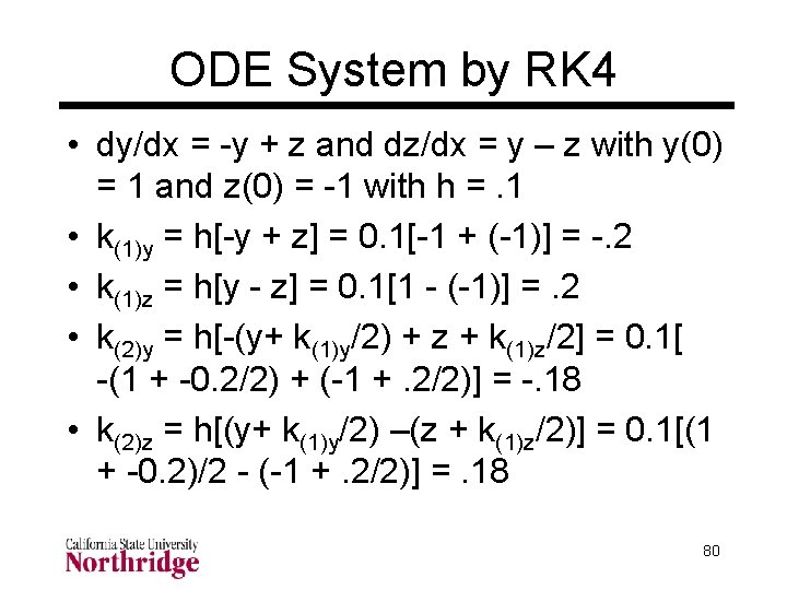
ODE System by RK 4 • dy/dx = -y + z and dz/dx = y – z with y(0) = 1 and z(0) = -1 with h =. 1 • k(1)y = h[-y + z] = 0. 1[-1 + (-1)] = -. 2 • k(1)z = h[y - z] = 0. 1[1 - (-1)] =. 2 • k(2)y = h[-(y+ k(1)y/2) + z + k(1)z/2] = 0. 1[ -(1 + -0. 2/2) + (-1 +. 2/2)] = -. 18 • k(2)z = h[(y+ k(1)y/2) –(z + k(1)z/2)] = 0. 1[(1 + -0. 2)/2 - (-1 +. 2/2)] =. 18 80

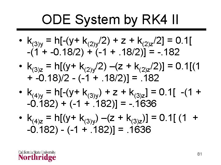
ODE System by RK 4 II • k(3)y = h[-(y+ k(2)y/2) + z + k(2)z/2] = 0. 1[ -(1 + -0. 18/2) + (-1 +. 18/2)] = -. 182 • k(3)z = h[(y+ k(2)y/2) –(z + k(2)z/2)] = 0. 1[(1 + -0. 18)/2 - (-1 +. 18/2)] =. 182 • k(4)y = h[-(y+ k(3)y) + z + k(3)z] = 0. 1[ -(1 + -0. 182) + (-1 +. 182)] = -. 1636 • k(4)z = h[(y+ k(3)y) –(z + k(3)z)] = 0. 1[ (1 + -0. 182) - (-1 +. 182)] =. 1636 81

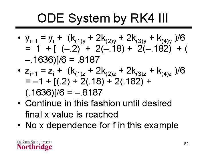
ODE System by RK 4 III • yi+1 = yi + (k(1)y + 2 k(2)y + 2 k(3)y + k(4)y )/6 = 1 + [ (–. 2) + 2(–. 182) + ( –. 1636)]/6 =. 8187 • zi+1 = zi + (k(1)z + 2 k(2)z + 2 k(3)z + k(4)z )/6 = – 1 + [(. 2) + 2(. 182) + (. 1636)]/6 = –. 8187 • Continue in this fashion until desired final x value is reached • No x dependence for f in this example 82

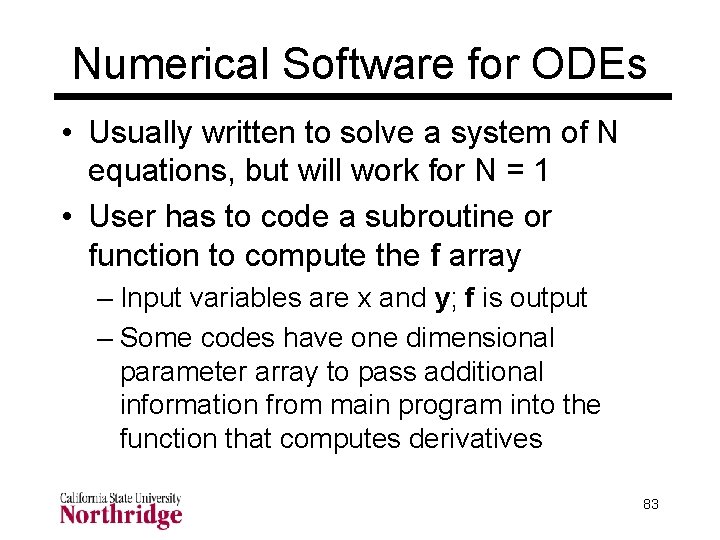
Numerical Software for ODEs • Usually written to solve a system of N equations, but will work for N = 1 • User has to code a subroutine or function to compute the f array – Input variables are x and y; f is output – Some codes have one dimensional parameter array to pass additional information from main program into the function that computes derivatives 83

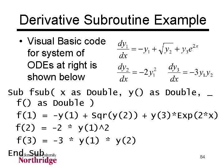
Derivative Subroutine Example • Visual Basic code for system of ODEs at right is shown below Sub fsub( x as Double, y() as Double, _ f() as Double ) f(1) = -y(1) + Sqr(y(2)) + y(3)*Exp(2*x) f(2) = -2 * y(1)^2 f(3) = -3 * y(1) * y(2) End Sub 84

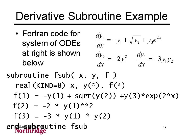
Derivative Subroutine Example • Fortran code for system of ODEs at right is shown below subroutine fsub( x, y, f ) real(KIND=8) x, y(*), f(*) f(1) = -y(1) + sqrt(y(2)) +y(3)*exp(2*x) f(2) = -2 * y(1)**2 f(3) = -3 * y(1) * y(2) end subroutine fsub 85

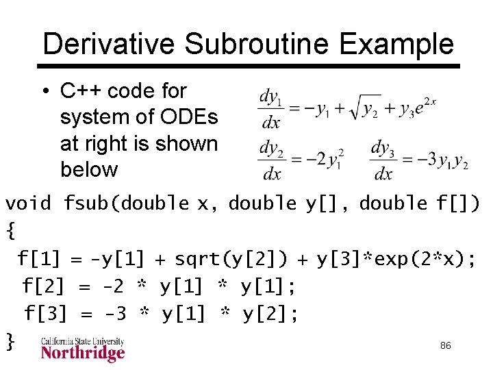
Derivative Subroutine Example • C++ code for system of ODEs at right is shown below void fsub(double x, double y[], double f[]) { f[1] = -y[1] + sqrt(y[2]) + y[3]*exp(2*x); f[2] = -2 * y[1]; f[3] = -3 * y[1] * y[2]; } 86