DRAINAGE DESIGN OF DRAINAGE SYSTEMS Lecture note compiled

DRAINAGE & DESIGN OF DRAINAGE SYSTEMS Lecture note compiled by: Dr. Durotimi John, Ph. D Associate Professor of Soil and Water Engineering

4. 1 INTRODUCTION Drainage means the removal of excess water from a given place. Two types of drainage can be identified: i) Land Drainage: This is large scale drainage where the objective is to drain surplus water from a large area by such means as excavating large open drains, erecting dykes and levees and pumping. Such schemes are necessary in low lying areas and are mainly Civil Engineering work.

ii) Field Drainage: This is the drainage that concerns us in agriculture. It is the removal of excess water from the root zone of crops.

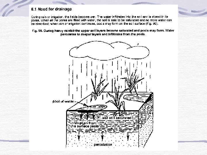
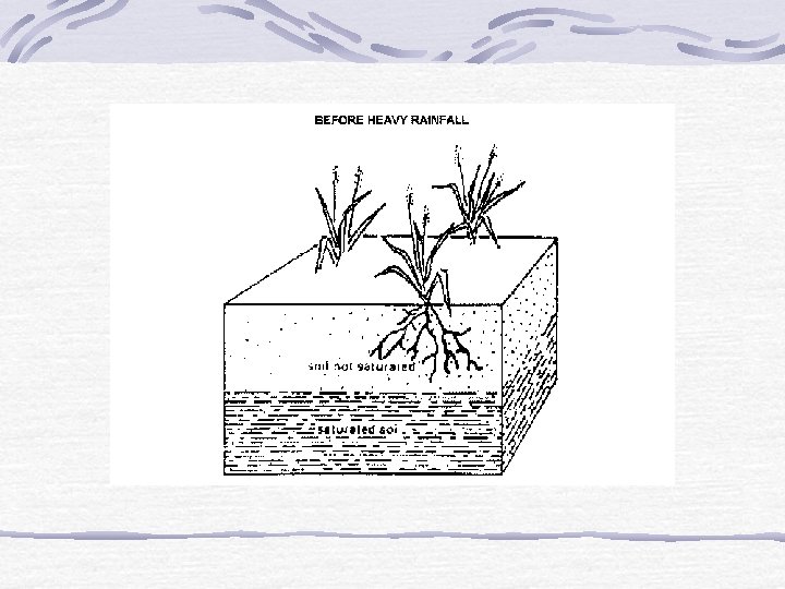
Water in Soil After Heavy Rain

The main aims of Field drainage include: i) To bring soil moisture down from saturation to field capacity. At field capacity, air is available to the soil and most soils are mesophites ie. like to grow at moisture less than saturation. ii) Drainage helps improve hydraulic conductivity: Soil structure can collapse under very wet conditions and so also engineering structures. iii) In some areas with salt disposition, especially in arid regions, drainage is used to leach excess salt.

The main aims of Field drainage Contd. iv) In irrigated areas, drainage is needed due to poor application efficiency which means that a lot of water is applied. v) Drainage can shorten the number of occasions when cultivation is held up waiting for soil to dry out.

Two types of drainage exist: Surface and Sub-surface drainage. 4. 2 DESIGN OF SURFACE DRAINAGE SYSTEMS: Surface drainage involves the removal of excess water from the surface of the soil. This is done by removing low spots where water accumulates by land forming or by excavating ditches or a combination of the two.

Surface Drainage

Surface Drainage Contd. Land forming is mechanically changing the land surface to drain surface water. This is done by smoothing, grading, bedding or leveling. Land smoothing is the shaping of the land to a smooth surface in order to eliminate minor differences in elevation and this is accomplished by filling shallow depressions. There is no change in land contour. Smoothing is done using land levelers or planes

Surface Drainage Concluded Land grading is shaping the land for drainage done by cutting, filling and smoothening to planned continuous surface grade e. g. using bulldozers or scrapers.

4. 2. 1 Design of Drainage Channels or Ditches 4. 2. 1. 1 Estimation of Peak Flows: This can be done using the Rational formula, Cook's method, Curve Number method, Soil Conservation Service method etc. Drainage coefficients (to be treated later) are at times used in the tropics especially in flat areas and where peak storm runoff would require excessively large channels and culverts. This may not apply locally because of high slopes.

a) The Rational Formula: It states that: Qp = (CIA)/360 where Qp is the peak flow (m 3 /s); C is dimensionless runoff coefficient; I is the rainfall intensity for a given return period. Return period is the average number of years within which a given rainfall event will be expected to occur at least once. A is the area of catchment (ha).

Using the Rational Method i) Obtain area of catchment by surveying or from maps or aerial photographs. ii) Estimate intensity using the curve in Hudson's Field Engineering, page 42. iii) The runoff coefficient C is a measure of the rain which becomes runoff. On a corrugated iron roof, almost all the rain would runoff so C = 1, while in a well drained soil, nine-tenths of the rain may soak in and so C = 0. 10. The table (see handout) from Hudson's Field Engineering can be used to obtain C value. Where the catchment has several different kinds of characteristics, the different values should be combined in proportion to the area of each.

Runoff Coefficient, C

b) Cook's Method: Three factors are considered: Vegetation, Soil permeability and Slope. These are the catchment characteristics. For each catchment, these are assessed and compared with Table 3. 4 of Hudson's Field Engineering

Table 3. 4: Hudson’s Field Eng’g (CC)

Example A catchment may be heavy grass (10) on shallow soils with impeded drainage(30) and moderate slope(10). Catchment characteristics (CC) is then the sum of the three ie. 50. The area of the catchment is then measured, and using the Area, A and the CC, the maximum runoff can be read from Table 3. 5 (Field Engineering, pp. 45).

Table 3. 5: Hudson’s Field Eng’g (Runoff Values)

Cook’s Method Contd. This gives the runoff for a 10 yr return period. For other return periods, other than 10 years, the conversion factor is: Return Period (yrs): 2 5 10 25 50 Conversion factor: 0. 90 0. 95 1. 00 1. 25 1. 50 Another factor to be considered is the shape of the catchment. Table 3. 5 gives the runoff for a catchment, which is roughly square or round. For other catchment shapes, the following conversion factors should be used: Square or round catchment (1) Long & narrow

Surface Drainage Channels The drainage channels are normally designed using the Manning formula. The required capacity of a drainage channel is calculated from the summation of the inflowing streams.

Surface Drainage Channels Contd. The bed level of an open drain collecting flow from field pipe drains should be such as to allow free fall from the pipe drain outlets under maximum flow conditions, with an allowance for siltation and weed growth. 300 mm is a reasonable general figure.

Surface Ditch Arrangements The ditch arrangement can be random, parallel or cross- slope. Random ditch system: Used where only scattered wet lands require drainage. Parallel ditch system: Used in flat topography. Ditches are parallel and perpendicular to the slope. Laterals, which run in the direction of the flow, collect water from ditches.

Surface Ditch Arrangements

4. 3 DESIGN OF SUB-SURFACE DRAINAGE SYSTEMS Sub-surface drainage is the removal of excess groundwater below the soil surface. It aims at increasing the rate at which water will drain from the soil, and so lowering the water table, thus increasing the depth of drier soil above the water table. Sub-surface drainage can be done by open ditches or buried drains.

Sub-Surface Drainage Using Ditches

Sub-Surface Drainage Using Ditches have lower initial cost than buried drains; There is ease of inspection and ditches are applicable in some organic soils where drains are unsuitable. Ditches, however, reduce the land available for cropping and require more maintenance that drains due to weed growth and erosion.

Sub-Surface Drains Using Buried Drains

Sub-Surface Drainage Using Buried Drains Buried drains refer to any type of buried conduits having open joints or perforations, which collect and convey drainage water. They can be fabricated from clay, concrete, corrugated plastic tubes or any other suitable material. The drains can be arranged in a parallel, herringbone, double main or random fashion.

Buried Drains

Arrangements of Sub-Surface Drains

Sub-Surface Drainage Designs The Major Considerations in Subsurface Drainage Design Include: Drainage Coefficient; Drain Depth and Spacing; Drain Diameters and Gradient; Drainage Filters.

Drainage Coefficient This is the rate of water removal used in drainage design to obtain the desired protection of crops from excess surface or sub-surface water and can be expressed in mm/day , m/day etc. Drainage is different in Rain-Fed Areas and Irrigated Areas

Drainage Coefficient in Rain -Fed Areas This is chosen from experience depending on rainfall. The following are guidelines. A. Table 4. 1 : Drainage Coefficient for Rain-Fed Areas* Mean annual rainfall Drainage coefficient (mm/day) (mm/yr) Ministry of Agric. Hudson 2000 25 20 1950 25 19. 5 1500 19 15 1000 13 10 875 10 < 875 7. 5 10. . . . . . . Source: *From Ministry of Agric. , U. K (1967) & Hudson (1975)

Other Methods For Obtaining Drainage Coefficient in Rain-Fed Areas Note: Hudson suggests that for MAR > 1000 mm, drainage coefficient is MAR/1000 mm/day and where MAR < 1000 mm, drainage coefficient is 10 mm/day. B. From rainfall records, determine peak rainfall with a certain probability depending on the value of crops or grounds to be protected e. g. 5 day rainfall for 1: 2 return period. C. Divide the rainfall of the heaviest rainfall month by the days of the month e. g. in St. Augustine, Trinidad, the heaviest rainfall month is August with 249 mm. i. e. Drainage discharge = 249/31 = 8. 03 mm/day. Use this method as a last resort.

Drainage Coefficient in Irrigated Areas In irrigated areas, water enters the groundwater from: Deep percolation, Leaching requirement, Seepage or Conveyance losses from watercourses and canals and Rainfall for some parts of the world.

Example 1 In the design of an irrigation system, the following properties exist: Soil field capacity is 28% by weight, permanent wilting point is 17% by weight; Bulk density = 1. 36 g/cm 3; root zone depth is 1 m; peak ET is 5 mm/day; irrigation efficiency is 60%, water conveyance efficiency is 80%, 50 % of water lost in canals contribute to seepage; rainfall for January is 69 mm and evapotranspiration is 100 mm; salinity of irrigation water is 0. 80 mm hos/cm while that acceptable is 4 mmhos/cm. Compute the drainage coefficient.

Solution: Readily available moisture (RAM) = ½ (FC - PWP) = 1/2(28 - 17) = 5. 5%. In depth, RAM = 0. 055 x 1. 36 x 1000 mm= 74. 8 mm = Net irrigation Shortest irrigation interval = RAM/peak ET = 74. 8/5 = 15 days With irrigation efficiency of 60 %, Gross irrigation requirement = 74. 8/0. 6 = 124. 7 mm. This is per irrigation. (a) Water losses = Gross - Net irrigation = 124. 7 - 74. 8 = 49. 9 mm Assuming 70% is deep percolation while 30% is wasted on the soil surface (Standard assumption), deep percolation = 0. 7 x 49. 9 = 34. 91 mm

Solution Contd. (b)Seepage Conveyance efficiency, Ec = Water delivered to farm Water released at dam = 0. 8 Water delivered to farm = Gross irrigation =124. 7 mm i. e. Water released = 124. 7/0. 8 = 155. 9 mm Excess water or water lost in canal = 155. 9 - 124. 7 = 31. 2 mm Since half of the water is seepage (given), the rest will be evaporation during conveyance Seepage = 1/2 x 31. 2 mm = 15. 6 mm

Solution Contd. (c) Leaching Reqd. = Ecirrig (ET - Rain ) = 0. 8 (100 -69) Ec accep 4 = 7. 75 mm This is for one month; for 15 days, we have 3. 88 mm (d) Rainfall = 69 mm; for 15 days, this is 34. 5 mm Note: In surface irrigation systems, deep percolation is much higher than leaching requirement so only the former is used in computation. It is assumed that excess water going down the soil as a result of deep percolation can be used for leaching. In sprinkler system, leaching requirement may be greater than deep percolation and can be used instead.

Solution Concluded Neglecting Leaching Requirement, Total water input into drains is equal to: 34. 91 + 15. 6 + 34. 5 = 85. 01 mm This is per 15 days, since irrigation interval is 15 days Drainage coefficient = 85. 01/15 = 5. 67 = 6 mm/day.

Drain Depth and Spacing L is drain spacing; h is mid drain water table height (m) above drain level; Do is depth of aquifer from drain level to impermeable layer(m); q is the water input rate(m/day) = specific discharge or drainage coefficient; K is hydraulic conductivity(m/day); H is the depth to water table.

Design Water table depth (H): This is the minimum depth below the surface at which the water table should be controlled and is determined by farming needs especially crop tolerance to water. Typically, it varies from 0. 5 to 1. 5 m.

Design Depth of Drain The deeper a drain is put, the larger the spacing and the more economical the design becomes. Drain depth, however, is constrained by soil and machinery limitations. Table : Typical Drain Depths(D) Soil Type Drain Depth (m) Sand 0. 6 Sandy loam 0. 8 - 1. 0 Silt loam 0. 8 - 1. 8 Clay loam 0. 6 - 0. 8 Peat 1. 2 - 1. 5

Drain Spacing (L) This is normally determined using the Hooghoudt equation. It states that Hooghoudt equation states that for ditches reaching the impermeable layer: L 2 = 8 K Do h + 4 K h q (See definitions of terms above) For tube drains which do not reach the impermeable layer, the equation can be modified as: L 2 = 8 K d h + 4 K h 2 q Where d is called the Houghoudt equivalent d. The equation for tube drains can be solved using trial and error method or the graphical method.

Example 2 For the drainage design of an irrigated area, drain pipes with a radius of 0. 1 m are used. They are placed at a depth of 1. 8 m below the soil surface. A relatively impermeable soil layer was found at a depth of 6. 8 m below the surface. From auger hole tests, the hydraulic conductivity above this layer was estimated as 0. 8 m/day. The average irrigation losses, which recharge the groundwater, are 40 mm per 20 days so the average discharge of the drain system amounts to 2 mm/day. Estimate the drain spacing, if the depth of the water table is 1. 2 m.

Solution

Solution Contd. Trial One Assume L = 75 m, from Houghout d table provided, with L = 75 m, and Do = 5 m, d = 3. 49 m. From equation (1), L 2 = (1920 x 3. 49) + 576 = 7276. 8; L = 85. 3 m Comment: The L chosen is small since 75 < 85. 3 m Try L = 100 m, from table, d = 3. 78 From (1), L 2 = (1920 x 3. 78) + 576 = 7833. 6 ; L = 88. 51 m Comment: Since 88. 51 < 100, try a smaller L; L should be between 75 and 100 m.

Analytical Solution Concluded Try L = 90 m, d =3. 49 + 15/25(3. 78 - 3. 49) = 3. 66 m L 2 = (1920 x 3. 66) + 576 = 7603. 2 m ; L = 87 m Comment: Since 87 < 90, try a smaller L; L should be between 75 and 90. Try L = 87 m, d = 3. 49 + 12/25(3. 78 - 3. 49) =3. 63 m L 2 = (1920 x 3. 63) + 576 = 7545. 6; L = 86. 87 m Comment: The difference between the assumed and calculated L is <1, so : Drain Spacing = 87 m.

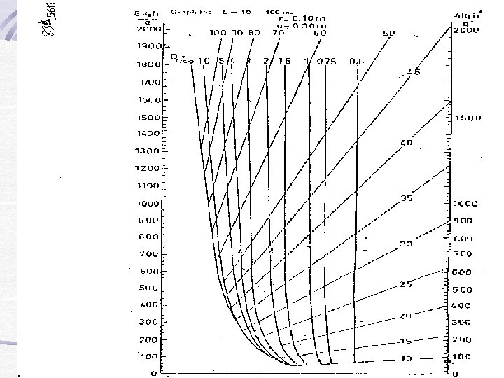
Graphical Solution Calculate 4 K h 2 and 8 K h q 4 K h 2 = 4 x 0. 8 x 0. 62 = 576; q 0. 002 8 K h = 8 x 0. 6 = 1920 q 0. 002 Locate the two points on graph given and join. For a value of Do = 5 m; produce downwards to meet the line. Read off the spacing on the diagram L = 87 m

Drain Diameters and Gradients There are two approaches to design: (a) Transport approach: Assumes that pipes are flowing full from top to end of field. Assumes uniform flow. (b) Drainage approach: Assumes that water enters the pipe all down the length as it is perforated. This is more realistic.

Parameters Required to use Solution Graphs (a) Types of pipes: Pipes can be smooth or rough. Clay tiles and smooth plastic pipes are smooth while corrugated plastic pipes are rough. (b) Drainable area: The area drained by one lateral and is equal to the maximum length of a lateral multiplied by drain spacing. The whole area drained by the laterals discharging into a collector represents the drainable area of the collector.

Parameters Required to use Solution Graphs Contd. c) Specific discharge: Earlier defined. Same as drainage coefficient. d) Silt safety factors: Used to account for the silting of pipes with time by making the pipes bigger. 60, 75 and 100 % pipe capacity factors are indicated. This means allowing 40, 25 and 0% respectively for silting. e) Average hydraulic gradient(%): normally the soil slope.

Example: The drainage design of a field is drain spacing = 30 m, length of drain lines = 200 m, slope = 0. 10%, specific discharge = 10 mm/day. Estimate drain diameter. Assume 60% silt factor and clay tiles. Solution: Area to be drained by one lateral = 30 m x 200 m = 6000 m 2 = 0. 6 ha Slope = average hydraulic gradient = 0. 10% ; Q = 10 mm/day Using chart for smooth drains, nearest diameter = 70 mm inside diameter.

4. 3. 4 Drainage Filters for tile drains are permeable materials eg. gravel placed around the drains for the purpose of improving the flow conditions in the area immediately surrounding the drains as well as for improving bedding conditions. Filters provide a high hydraulic conductivity around the drains which stabilizes the soil around and prevent small particles from entering the lateral drains since they are perforated.

Soils that Need Filters a) Uniform soils will cause problems while non-uniform ones since they are widely distributed stabilize themselves. b) Clays have high cohesion so cannot be easily moved so require no filters. c) Big particles like gravel can hardly be moved due to their weight. * Fine soils are then the soils that will actually need filters especially if they are uniform.

Drainage Filters Continued a) Filters are needed to be gravel with same uniformity with the soil to be protected. b) D 15 Filter < 5 D 85 Soil ; D 15 Filter < 20 D 15 Soil ; D 50 Filter < 25 D 50 Soil. These are the filtration criteria. To give adequate hydraulic conductivity, D 85 Filter > 5 D 15 Soil. These criteria are difficult to achieve and should serve as guidelines.

Laying Plastic Pipes: A Trench is excavated, the pipe is laid in the trench, permeable fill is added, and then the trench is filled. This is for smooth-walled rigid plastic pipes or tile drains. A Flexible Corrugated Pipe can be laid by machines, which lay the pipes without excavating an open trench (trench less machines).

Practical assignments 1 1. compute the drainage coefficient for design of open ditch system as surface drainage means for draining 1500 ha. watershed area, if (i) Run-off is entering the watershed at 4. 5 m 3/s for 3 hours period (ii) Total rainfall during 24 hours duration is 8. 5 cm (iii) Infiltration loss during 24 hours duration is 1. 5 cm (iv) Crop water tolerance depth is 8 cm

Practical assignment 2 A). Design an open drain of trapezoidal section for draining 500 ha. land with the following information: (i) Drainage coefficient is 3. 0 cm (ii) Maximum bed slope is 0. 15% (iii) Soil of area is silt (iv) Depth of drain is 1. 50 cm B). Determine the percentage increase in discharge capacity of open ditch constructed for draining the area of 1500 ha. land if the drainage coefficient increase from 1. 5 to 3. 0 cm.