Speeding Up MRF Optimization using Graph Cuts for

Speeding Up MRF Optimization using Graph Cuts for Computer Vision Vibhav Vineet Adviser: Prof. P. J. Narayanan

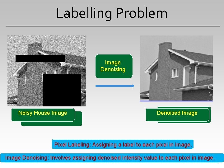
Labelling Problem Extracting Disparity Image Foreground map Denoising calculation Pixels Left Noisy Tsukuba House Image Flower Image Extracting Denoised Disparity Image Map Foreground Object Pixel Labeling: Assigning a label to each pixel in image. Image. Denoising: Segmentation: Involves assigning Separating denoised Foreground value layer from to each background pixelright in image. layer Stereo Correspondence: Involves Calculation ofintensity depth map using left and images

Labelling Problem - MAP Estimation To find the best possible configuration. -But the complexity increases -With the number of variables/pixels - With the number of labels in the label set -Using joint probability or conditional probabilities to evaluate the best possible configuration - Very hard with the limited computation and memory power -Energy minimization method - MAP – MRF equiivalence - Methods provide approximate solution at a moderate times - Generally, in computer vision an energy function involve unary cost and pairwise interactions between variables.

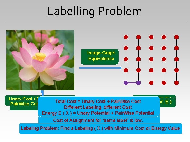
Labelling Problem Image-Graph Equivalence Graph G( V, E ) Unary Cost ( Per Vertex Cost) Total Cost = Unary Cost + Pair. Wise Cost. Graph G( V, E ) Pair. Wise Cost ( Per Edge Cost ) Different Labeling, different Cost Energy E ( X ) = Unary Potential + Pair. Wise Potential of Assignment for “fg”label” is low. Cost of Assignment for “same is low. Cost of Assignment for “bg” is high. Cost of Assignment “different labels” is. Cost high. or Energy Value Labeling Problem: Find a Labelingfor( X ) with Minimum

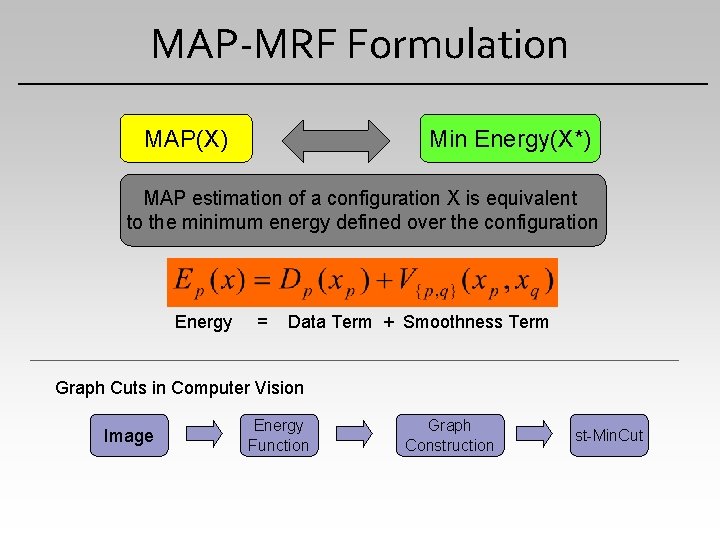
MAP-MRF Formulation MAP(X) Min Energy(X*) MAP estimation of a configuration X is equivalent to the minimum energy defined over the configuration Energy = Data Term + Smoothness Term Graph Cuts in Computer Vision Image Energy Function Graph Construction st-Min. Cut

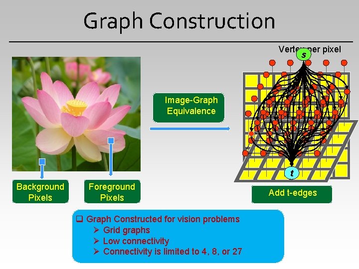
Graph Construction Vertex per pixel s Image-Graph Equivalence t Background Pixels Foreground Pixels q Graph Constructed for vision problems Ø Grid graphs Ø Low connectivity Ø Connectivity is limited to 4, 8, or 27 Graph Add. Image n-edges t-edges G(V, E)

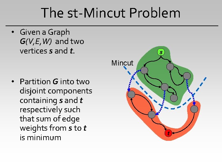
The st-Mincut Problem • Given a Graph G(V, E, W) and two vertices s and t. s Mincut • Partition G into two disjoint components containing s and t respectively such that sum of edge weights from s to t is minimum t

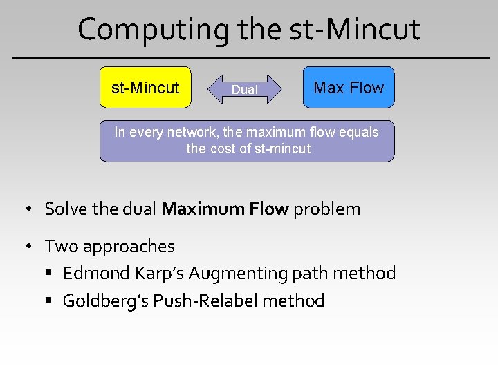
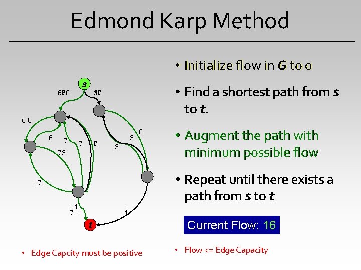
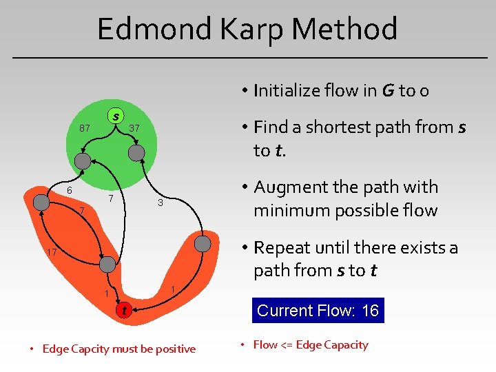
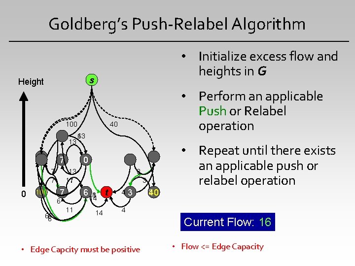
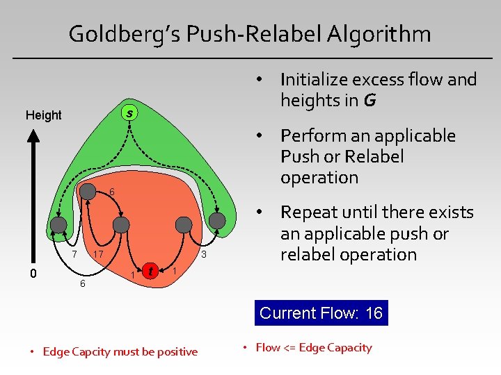
Computing the st-Mincut Dual Max Flow In every network, the maximum flow equals the cost of st-mincut • Solve the dual Maximum Flow problem • Two approaches Edmond Karp’s Augmenting path method Goldberg’s Push-Relabel method

Edmond Karp Method • Initialize flow in G to 0 s 100 93 87 • Find a shortest path from s to t. 40 37 60 6 7 7 7 0 13 7 3 0 3 • Augment the path with minimum possible flow • Repeat until there exists a path from s to t 17 11 14 71 1 4 t • Edge Capcity must be positive Current Flow: 10 0 3 16 • Flow <= Edge Capacity

Edmond Karp Method • Initialize flow in G to 0 s 87 6 • Find a shortest path from s to t. 37 7 • Augment the path with minimum possible flow 3 7 • Repeat until there exists a path from s to t 17 1 1 t • Edge Capcity must be positive Current Flow: 16 • Flow <= Edge Capacity

Goldberg’s Push-Relabel Algorithm • Initialize excess flow and heights in G s Height 40 100 7 0 100 87 87 7 0 13 100 13 6 6 7 0 0 7 3 3 0 6 11 40 37 3 0 13 11 17 6 66 6 • Perform an applicable Push or Relabel operation 8 1 14 14 t 43 1 0 3 340 • Repeat until there exists an applicable push or relabel operation 4 • Edge Capcity must be positive Current Flow: 9 0 16 • Flow <= Edge Capacity

Goldberg’s Push-Relabel Algorithm s Height 0 • Perform an applicable Push or Relabel operation 6 87 0 • Initialize excess flow and heights in G 0 17 6 37 3 1 t • Repeat until there exists an applicable push or relabel operation 1 Current Flow: 16 • Edge Capcity must be positive • Flow <= Edge Capacity

Motivation • Fast Computation Required • Robot navigation, surveillance, video processing etc • Video Processing at real time • • Large images Processing • • You tube and other web-servers Even our offshelf cameras take high resolution images Interactive tools

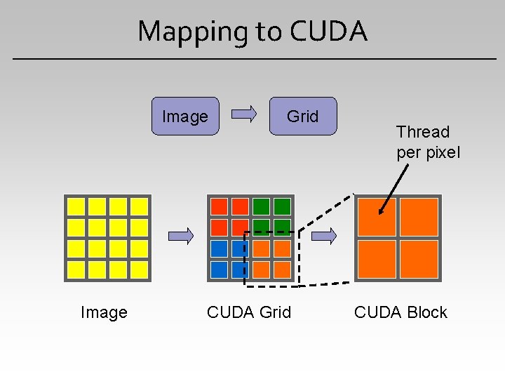
Mapping to CUDA Image Grid CUDA Grid Thread per pixel CUDA Block

Push-Relabel Algorithm on CUDA • Push is an local operation with each node sending flows to its neighbors. • Relabel is also a local operation, each vertex updates its own height. • Problems faced: Read After Write consistency Synchronization of threads

Handling Problems using Atomics • Push operations can performed without any read after write inconsistencies • Relabel is a per vertex operation • Employing atomic Capabilities and combining the push and pull kernels Push Kernel Relabel Kernel • Lowers Global memory access, empirically faster convergence is observed.

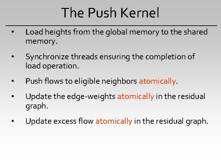
The Push Kernel • Load heights from the global memory to the shared memory. • Synchronize threads ensuring the completion of load operation. • Push flows to eligible neighbors atomically. • Update the edge-weights atomically in the residual graph. • Update excess flow atomically in the residual graph.

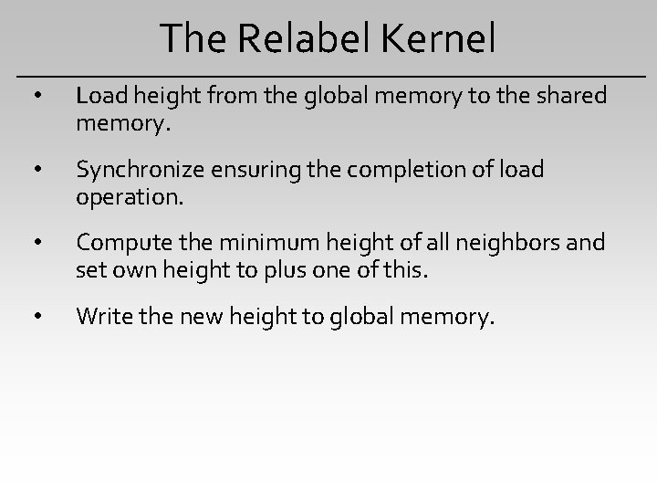
The Relabel Kernel • Load height from the global memory to the shared memory. • Synchronize ensuring the completion of load operation. • Compute the minimum height of all neighbors and set own height to plus one of this. • Write the new height to global memory.

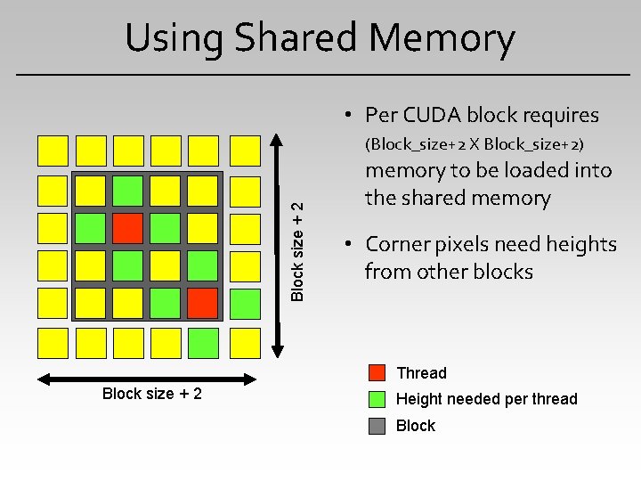
Using Shared Memory • Per CUDA block requires Block size + 2 (Block_size+2 X Block_size+2) memory to be loaded into the shared memory • Corner pixels need heights from other blocks Thread Block size + 2 Height needed per thread Block

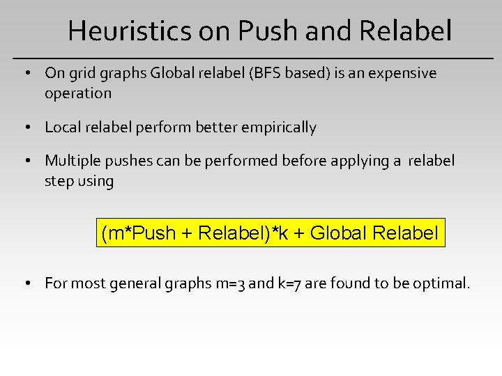
Heuristics on Push and Relabel • On grid graphs Global relabel (BFS based) is an expensive operation • Local relabel perform better empirically • Multiple pushes can be performed before applying a relabel step using (m*Push + Relabel)*k + Global Relabel • For most general graphs m=3 and k=7 are found to be optimal.

Stochastic Cuts • MRF consists of simple and difficult pixels. • Simple pixels get their correct labels in few initial iterations • Difficult (few) pixels exchange flows with their neighbors in later iterations • Stochastic Cuts processes pixels based on their activity • Activity is based on change in flows from previous to current iteration. Low activity is observed for simple pixels • Heuristically process simple pixels after a fixed number of iterations

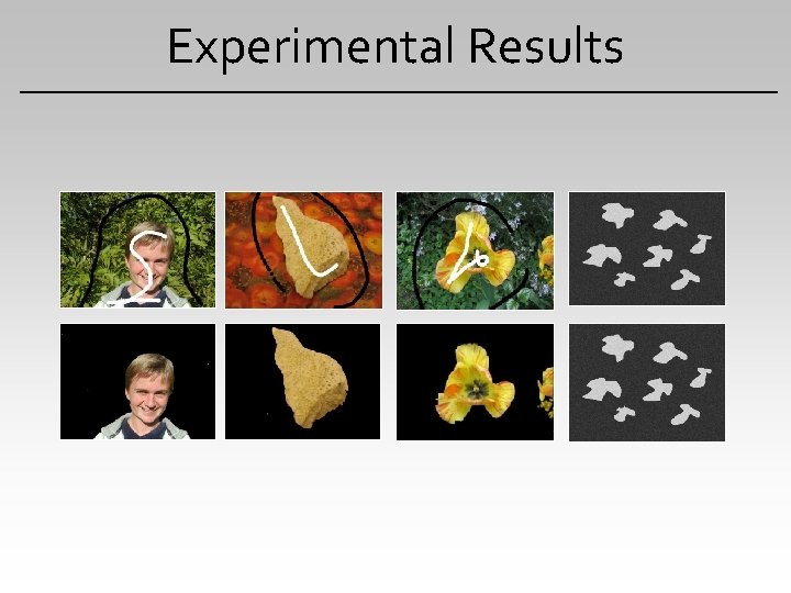
Experimental Results

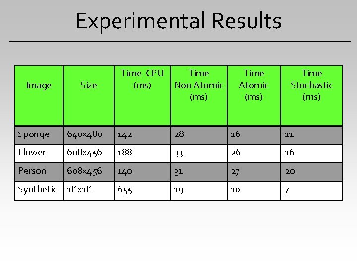
Experimental Results Image Size Time CPU (ms) Time Non Atomic (ms) Time Stochastic (ms) Sponge 640 x 480 142 28 16 11 Flower 608 x 456 188 33 26 16 Person 608 x 456 140 31 27 20 Synthetic 1 Kx 1 K 655 19 10 7

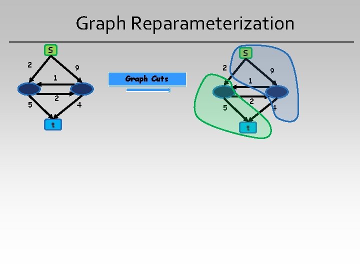
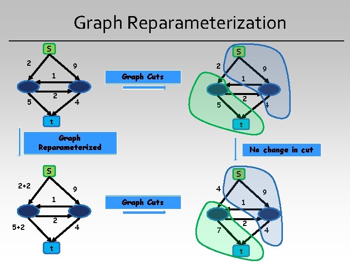
Graph Reparameterization S S 2 9 1 5 2 t 4 2 Graph Cuts 9 1 5 2 t 4

Graph Reparameterization S S 2 9 1 2 5 2 9 Graph Cuts 4 1 2 5 t t Graph Reparameterized No change in cut S S 2+2 4 9 1 5+2 4 2 t Graph Cuts 4 9 1 7 2 t 4

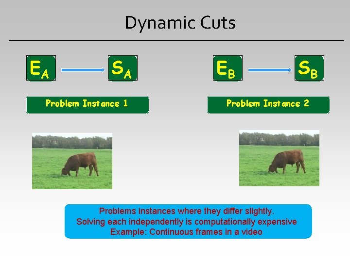
Dynamic Cuts EA SA Problem Instance 1 EB SB Problem Instance 2 Problems instances where they differ slightly. Solving each independently is computationally expensive Example: Continuous frames in a video

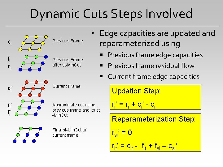
Dynamic Cuts Steps Involved • Edge capacities are updated and reparameterized using ci Previous Frame fi ri Previous Frame after st-Min. Cut ci’ Current Frame ri’ fi’ Approximate cut using previous frame and its st -Min. Cut Final st-Min. Cut of current frame Previous frame edge capacities Previous frame residual flow Current frame edge capacities Updation Step: ri ’ = r i + c i ’ - c i Reparameterization Step: rsi’ = 0 rit’ = cit - fit + fsi – csi’

Dynamic Cuts are parallizable • Updation and Reparameterization are independent and parallizable operations, work locally at every vertex. • st-Mincut is performed using a parallel implementation of Push Relabel algorithm.

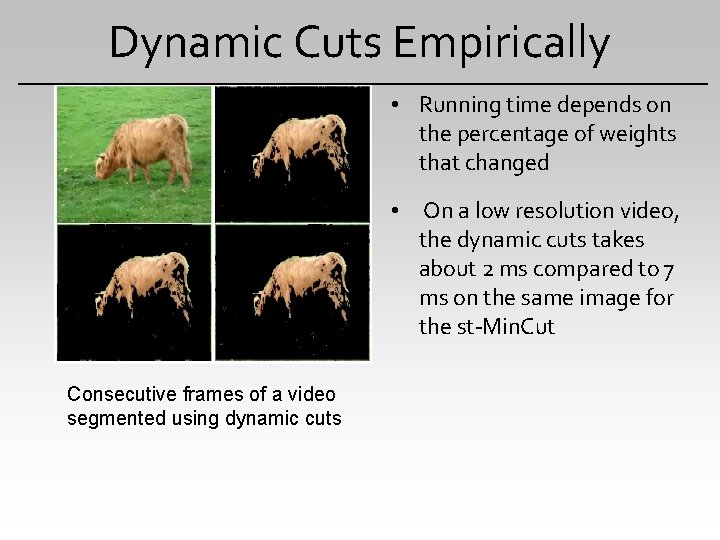
Dynamic Cuts Empirically • Running time depends on the percentage of weights that changed • On a low resolution video, the dynamic cuts takes about 2 ms compared to 7 ms on the same image for the st-Min. Cut Consecutive frames of a video segmented using dynamic cuts

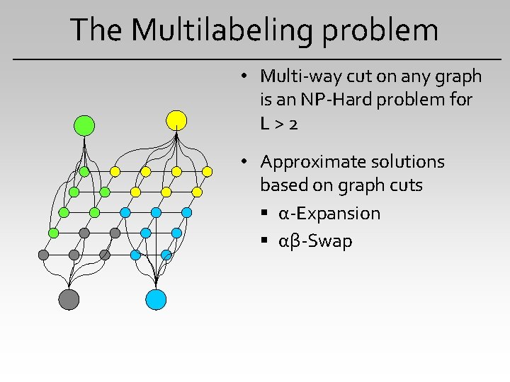
The Multilabeling problem • Multi-way cut on any graph is an NP-Hard problem for L>2 • Approximate solutions based on graph cuts α-Expansion αβ-Swap

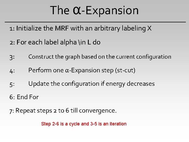
The α-Expansion 1: Initialize the MRF with an arbitrary labeling X 2: For each label alpha in L do 3: Construct the graph based on the current configuration 4: Perform one α-Expansion step (st-cut) 5: Update the configuration if energy decreases 6: End For 7: Repeat steps 2 to 6 till convergence. Step 2 -6 is a cycle and 3 -5 is an iteration

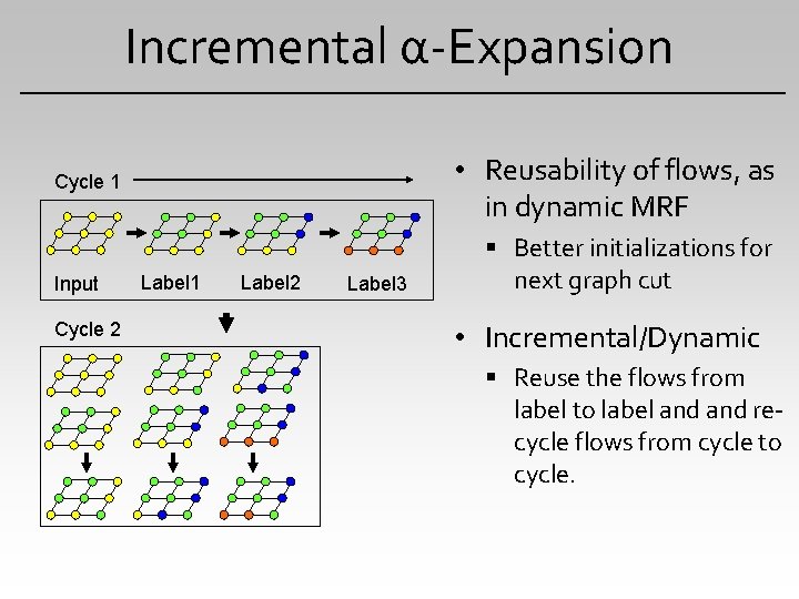
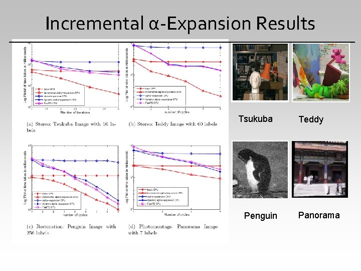
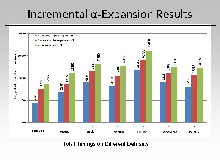
Incremental α-Expansion • Reusability of flows, as in dynamic MRF Cycle 1 Input Cycle 2 Label 1 Label 2 Label 3 Better initializations for next graph cut • Incremental/Dynamic Reuse the flows from label to label and recycle flows from cycle to cycle.

Incremental α-Expansion Results Tsukuba Penguin Teddy Panorama

Incremental α-Expansion Results Total Timings on Different Datasets

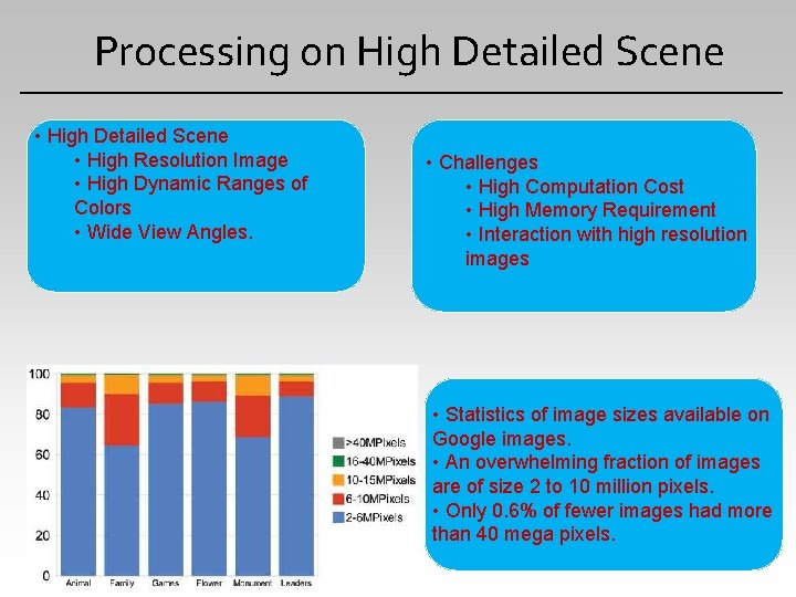
Processing on High Detailed Scene • High Resolution Image • High Dynamic Ranges of Colors • Wide View Angles. • Challenges • High Computation Cost • High Memory Requirement • Interaction with high resolution images • Statistics of image sizes available on Google images. • An overwhelming fraction of images are of size 2 to 10 million pixels. • Only 0. 6% of fewer images had more than 40 mega pixels.

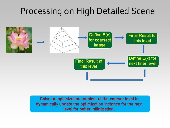
Processing on High Detailed Scene Define E(x) for coarsest image Final Result at this level Final Result for this level Define E(x) for next finer level Solve an optimization problem at the coarser level to dynamically update the optimization instance for the next level for better initialization.

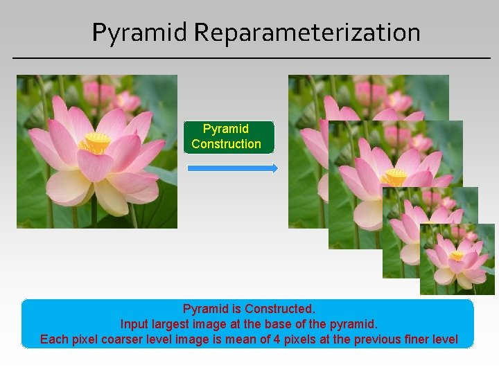
Pyramid Reparameterization Pyramid Construction Pyramid is Constructed. Input largest image at the base of the pyramid. Each pixel coarser level image is mean of 4 pixels at the previous finer level

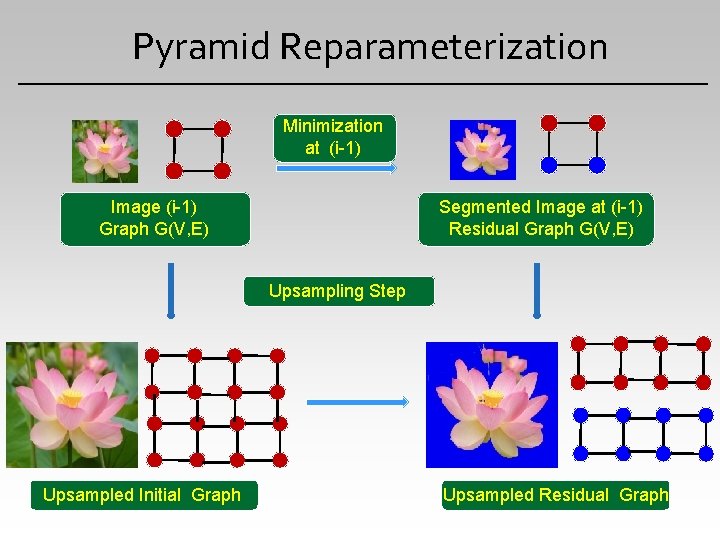
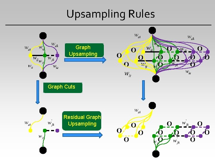
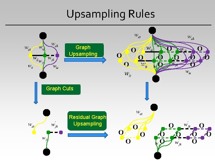
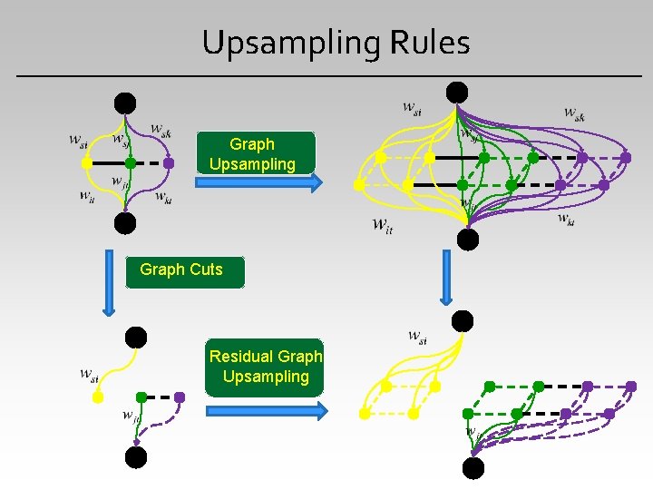
Pyramid Reparameterization Minimization at (i-1) Image (i-1) Graph G(V, E) Segmented Image at (i-1) Residual Graph G(V, E) Upsampling Step Upsampled Initial Graph Upsampled Residual Graph

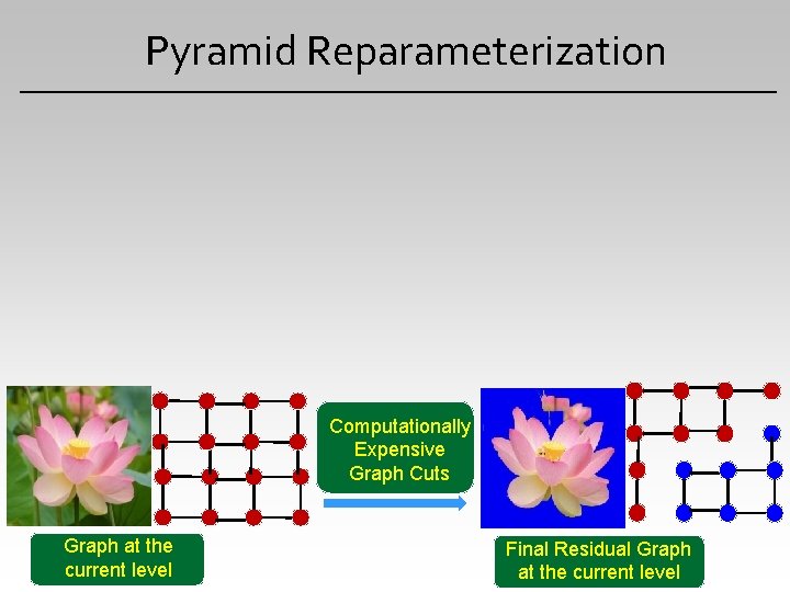
Pyramid Reparameterization Computationally Expensive Graph Cuts Graph at the current level Final Residual Graph at the current level

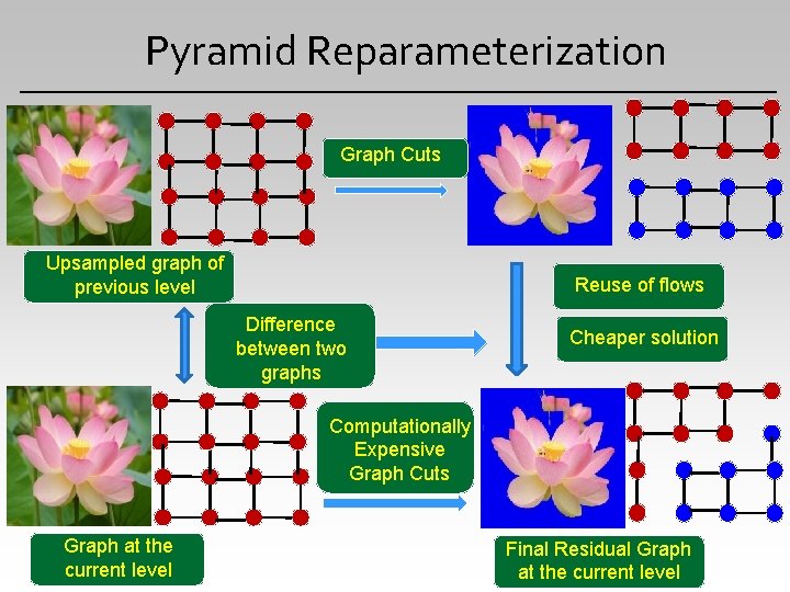
Pyramid Reparameterization Graph Cuts Upsampled graph of previous level Reuse of flows Difference between two graphs Cheaper solution Computationally Expensive Graph Cuts Graph at the current level Final Residual Graph at the current level

Upsampling Rules Graph Upsampling Graph Cuts Residual Graph Upsampling

Upsampling Rules Graph Upsampling Graph Cuts Residual Graph Upsampling

Upsampling Rules Graph Upsampling Graph Cuts Residual Graph Upsampling

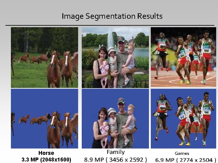
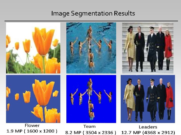
Image Segmentation Results Horse 3. 3 MP (2048 x 1600)

Image Segmentation Results

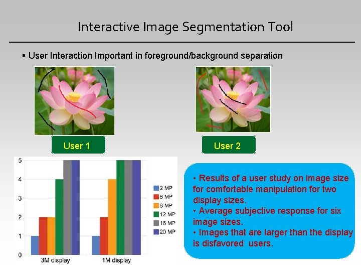
Interactive Image Segmentation Tool User Interaction Important in foreground/background separation User 1 User 2 • Results of a user study on image size for comfortable manipulation for two display sizes. • Average subjective response for six image sizes. • Images that are larger than the display is disfavored users.

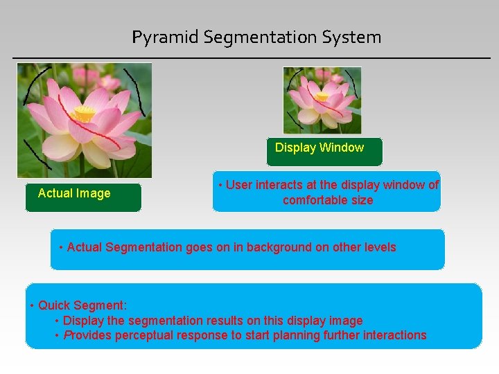
Pyramid Segmentation System Display Window Actual Image • User interacts at the display window of comfortable size • Actual Segmentation goes on in background on other levels • Quick Segment: • Display the segmentation results on this display image • Provides perceptual response to start planning further interactions

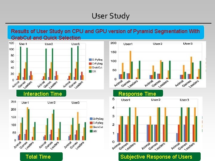
User Study Results of User Study on CPU and GPU version of Pyramid Segmentation With Grab. Cut and Quick Selection Interaction Time Total Time Response Time Subjective Response of Users

Multiresolution alpha-expansion - Build pyramid of graphs. - Perform alpha-expansion at a lower resolution graph. - Save the initial and final residual graphs for all the labels. - Upsample and reparameterize the previous resolution initial and final graphs and current resolution initial graph. - Perform alpha-expansion at this level. - Repeat this for all the levels in the pyramid.

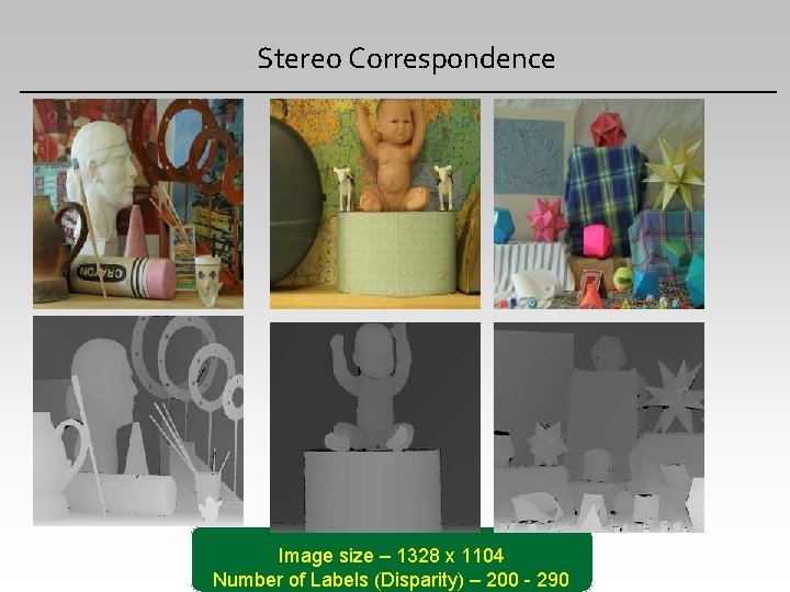
Stereo Correspondence Image size – 1328 x 1104 Number of Labels (Disparity) – 200 - 290

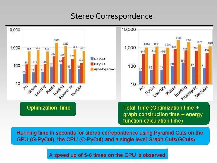
Stereo Correspondence Optimization Time Total Time (Optimization time + graph construction time + energy function calculation time) Running time in seconds for stereo correpondence using Pyramid Cuts on the GPU (G-Py. Cut), the CPU (C-Py. Cut) and a single level Graph Cuts(GCuts). A speed up of 5 -6 times on the CPU is observed.

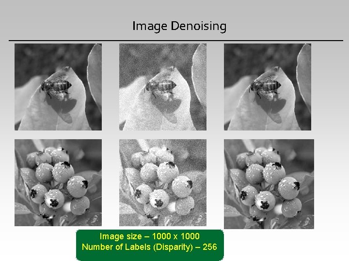
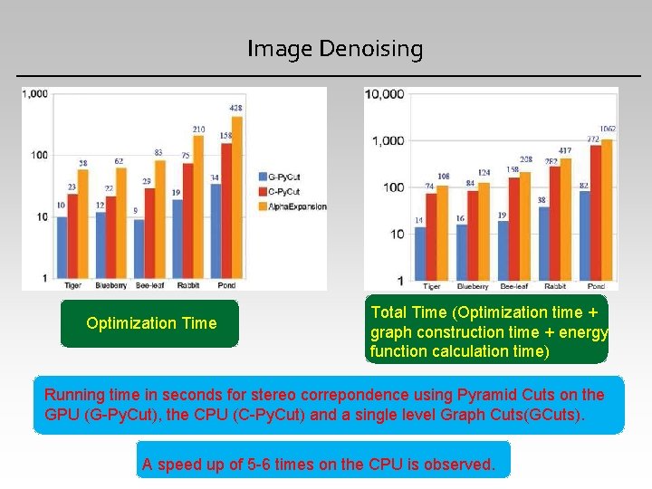
Image Denoising Image size – 1000 x 1000 Number of Labels (Disparity) – 256

Image Denoising Optimization Time Total Time (Optimization time + graph construction time + energy function calculation time) Running time in seconds for stereo correpondence using Pyramid Cuts on the GPU (G-Py. Cut), the CPU (C-Py. Cut) and a single level Graph Cuts(GCuts). A speed up of 5 -6 times on the CPU is observed.

Future Work • Higher order Interactions of variables in MRF • Computationally more challenging • Modelling this on our hierarchical and multiresolution framework • Using multiple GPUs to parallelize the alpha-expansion • Better interactive tools: • Both global and local interactions

Conclusion • Two methods to optimize basic graph cuts algorithm • Using facilities provided by parallel accelerators like GPU • Modelling graph cuts on hierarchical and dynamic framework for better initialization • Graph Cuts methods proved very instrumental solving many computationally challenging problems • Successes of graph cuts -> Promising future in the realm of energy minimization methods

Related Publications P. J. Narayanan, Vibhav Vineet and Timo Stitch. Fast Graph Cuts on the GPU Computing Gems (GCG), Volume 1 Dec. 2010 (Book Chapter). • Vibhav Vineet and P. J. Narayanan. Solving Multi-label MRFs using incremental alphaexpansion move on the GPUs. In Proceeding of Ninth Asian Conference on Computer Vision. (ACCV-2009), China, 2009. • Vibhav Vineet and P. J. Narayanan. CUDA Cuts: Fast Graph Cuts on the GPU. In Proceeding of CVPR workshop on Visual Computer Vision on GPUs (CVGPU-2008), Alaska, USA, 2008. • Vibhav Vineet, Pawan Harish, Suryakant Patidar and P. J. Narayanan. Fast Minimum Spanning Tree for Large Graphs on the GPU. In Proceeding of ACM SIGGRAPH High Performance Graphics (HPG-2009), New Orleans, LA, USA, 2009. • Pawan Harish, Vibhav Vineet and P. J. Narayanan. Large Graph Algorithms for Massively Multithreaded Architectures. IIIT Tech Report, IIIT/TR/2009/74. • CUDA Cuts: Fast Graph Cuts on the GPU. http: //cvit. iiit. ac. in/index. php? page=resources. (Software). Vibhav Vineet, Pawan Harish, Suryakant Patidar and P. J. Narayanan. Fast Minimum Spanning Tree for Large Graphs on the GPU Computing Gems (GCG). (Book Chapter).

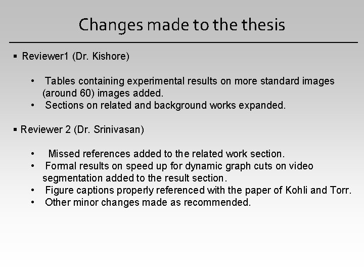
Changes made to thesis Reviewer 1 (Dr. Kishore) • Tables containing experimental results on more standard images (around 60) images added. • Sections on related and background works expanded. Reviewer 2 (Dr. Srinivasan) • • Missed references added to the related work section. Formal results on speed up for dynamic graph cuts on video segmentation added to the result section. • Figure captions properly referenced with the paper of Kohli and Torr. • Other minor changes made as recommended.

Thank You