Predictive Learning on Data Streams Haixun Wang 1

Predictive Learning on Data Streams Haixun Wang 1 and Ying Yang 2 1 IBM T. J. Watson Research Center 2 Monash University

Please find the latest version of this tutorial at: http: //wis. cs. ucla. edu/~hxwang/tutorial. ppt

Outline • Challenges – Volume, Speed, Time varying distribution • Part I: Learning models from streams – Accuracy, Efficiency – Intelligent model reusing • Part II: Applying models on streams – Efficiency, Accuracy – Intelligent load shedding

Background • Many real-life data are data streams in nature: – data from large number of embedded sensors – high-speed real-time financial and retailer data – large-volume network traffic data • Resources are limited – CPU cycles, bandwidth, and memory • Resource allocation is a very important issue.

Challenges in Classifying Streams • Cost of learning a model – impossible to mine the entire data at one time – can only afford constant memory per data sample • Concept Drifts – previously learned models are invalid – model updates can be costly • Cost of applying a model – classify data without seeing it?

PART I Learning Classifiers from Streams Issues: Accuracy, Cost, Model Reuse

Methods for Classifying Streams • • • Decision Tree Hoeffding Trees VFDT and CVFDT Ensemble of Classifiers etc.

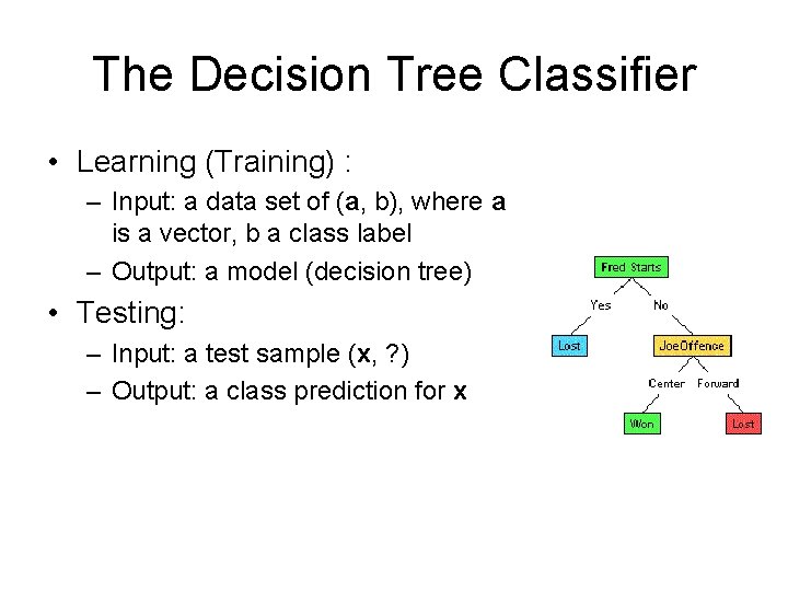
The Decision Tree Classifier • Learning (Training) : – Input: a data set of (a, b), where a is a vector, b a class label – Output: a model (decision tree) • Testing: – Input: a test sample (x, ? ) – Output: a class prediction for x

The Decision Tree Classifier • A divide-and-conquer approach – Simple algorithm, intuitive model – No ‘optimal’ model • Compute information gain for data in each node – Super-linear complexity • Typically a decision tree grows one level for each scan of data – Multiple scans are required • The data structure is not ‘stable’ – Subtle changes of data can cause global changes in the data structure

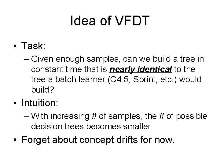
Idea of VFDT • Task: – Given enough samples, can we build a tree in constant time that is nearly identical to the tree a batch learner (C 4. 5, Sprint, etc. ) would build? • Intuition: – With increasing # of samples, the # of possible decision trees becomes smaller • Forget about concept drifts for now.

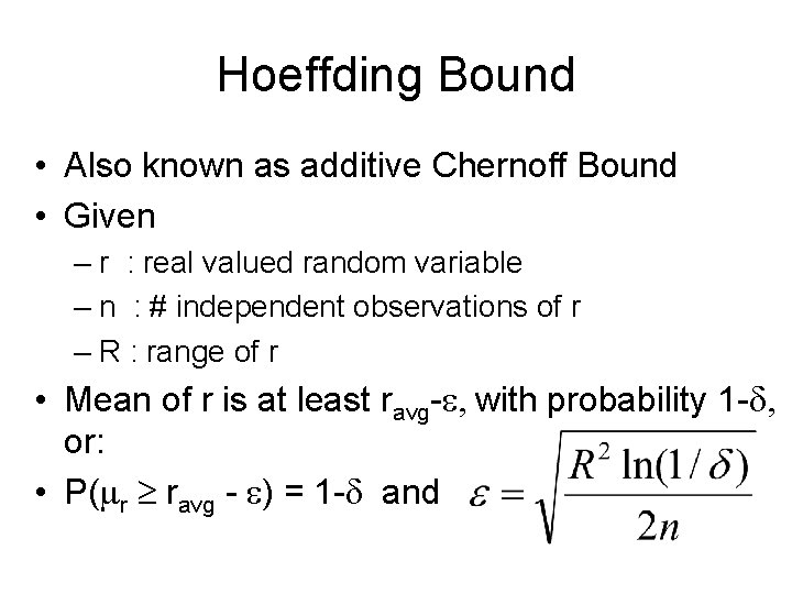
Hoeffding Bound • Also known as additive Chernoff Bound • Given – r : real valued random variable – n : # independent observations of r – R : range of r • Mean of r is at least ravg- , with probability 1 - , or: • P( r ravg - ) = 1 - and

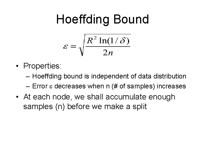
Hoeffding Bound • Properties: – Hoeffding bound is independent of data distribution – Error decreases when n (# of samples) increases • At each node, we shall accumulate enough samples (n) before we make a split

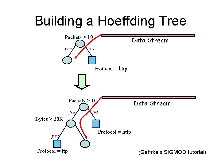
Building a Hoeffding Tree Packets > 10 yes Data Stream no Protocol = http Packets > 10 yes Data Stream no Bytes > 60 K yes Protocol = ftp Protocol = http (Gehrke’s SIGMOD tutorial)

Nearly Identical? • Categorical attributes – with a high probability, the attribute we choose for split is the same attribute as would be chosen by a batch learner – identical decision tree • Continuous attributes – discretize them into categorical ones

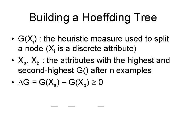
Building a Hoeffding Tree • G(Xi) : the heuristic measure used to split a node (Xi is a discrete attribute) • Xa, Xb : the attributes with the highest and second-highest G() after n examples • G = G(Xa) – G(Xb) 0

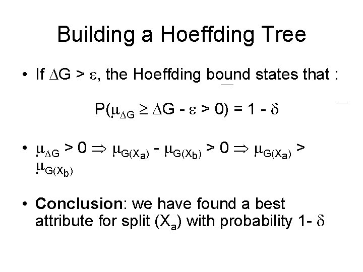
Building a Hoeffding Tree • If G > , the Hoeffding bound states that : P( G G - > 0) = 1 - • G > 0 G(Xa) - G(Xb) > 0 G(Xa) > G(Xb) • Conclusion: we have found a best attribute for split (Xa) with probability 1 -

Hoeffding Tree: Pros and Cons • Scales better than traditional DT algorithms – Incremental – Sub-linear with sampling – Small memory requirement • Cons: – – Only consider top 2 attributes Tie breaking takes time Grow a deep tree takes time Discrete attribute only

VFDT • Very Fast Decision Tree – Domingos, Hulten, 2000 • Various Improvement over Hoeffding Tree – Break near-ties more aggressively – G computed every nmin tuples (instead of for every tuple) – Deactivating unpromising leaf nodes – Dropping poor attributes –… – Better time and memory performance • Still does not handle concept drifts

Concept Drifts • Time-changing data streams • Incorporate new samples and eliminate effect of old samples • Naïve approach – Place a sliding window on the stream – Reapply C 4. 5 or VFDT whenever window moves – Time consuming!

CVFDT • Concept-adapting VFDT – Hulten, Spencer, Domingos, 2001 • Goal – Classifying concept-drifting data streams • Approach – – Make use of Hoeffding bound Incorporate “windowing” Monitor changes of information gain for attributes. If change reaches threshold, generate alternate subtree with new “best” attribute, but keep on background. – Replace if new subtree becomes more accurate.

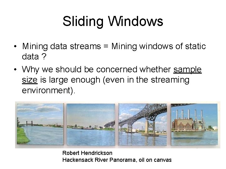
Sliding Windows • Mining data streams = Mining windows of static data ? • Why we should be concerned whether sample size is large enough (even in the streaming environment). Robert Hendrickson Hackensack River Panorama, oil on canvas

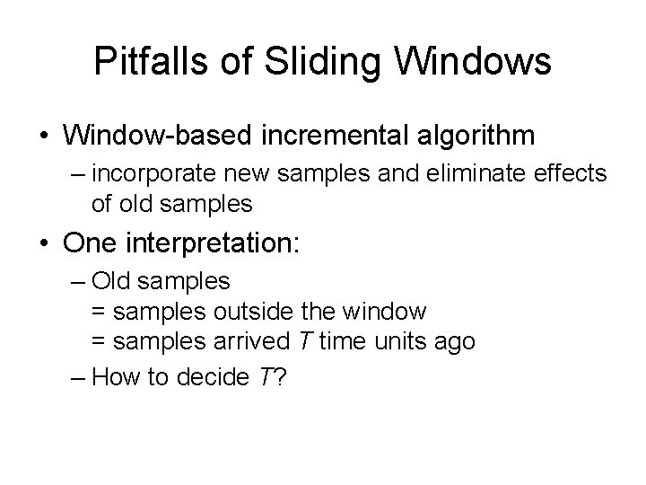
Pitfalls of Sliding Windows • Window-based incremental algorithm – incorporate new samples and eliminate effects of old samples • One interpretation: – Old samples = samples outside the window = samples arrived T time units ago – How to decide T?

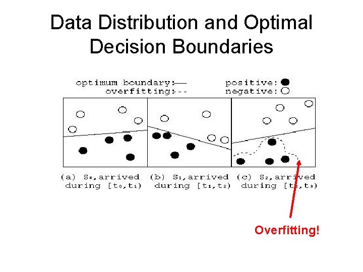
Data Distribution and Optimal Decision Boundaries Overfitting!

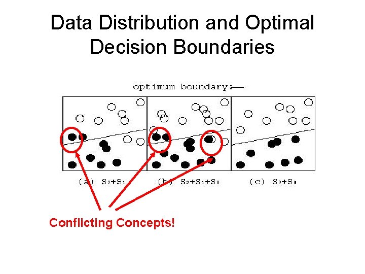
Data Distribution and Optimal Decision Boundaries Conflicting Concepts!

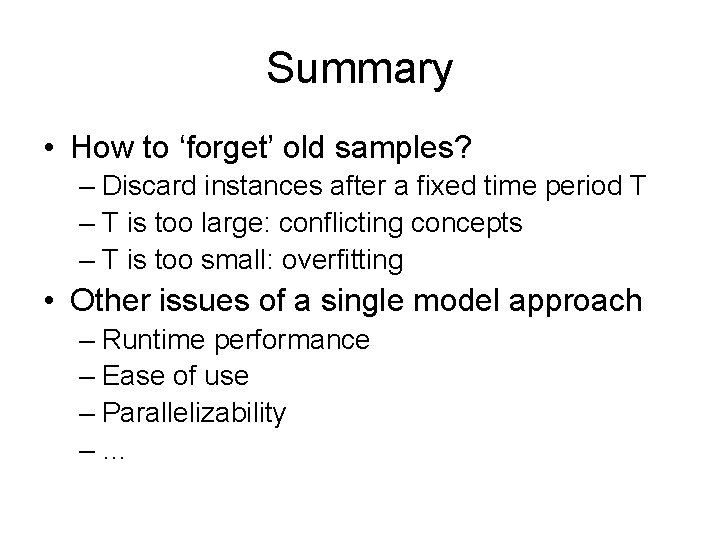
Summary • How to ‘forget’ old samples? – Discard instances after a fixed time period T – T is too large: conflicting concepts – T is too small: overfitting • Other issues of a single model approach – Runtime performance – Ease of use – Parallelizability –…

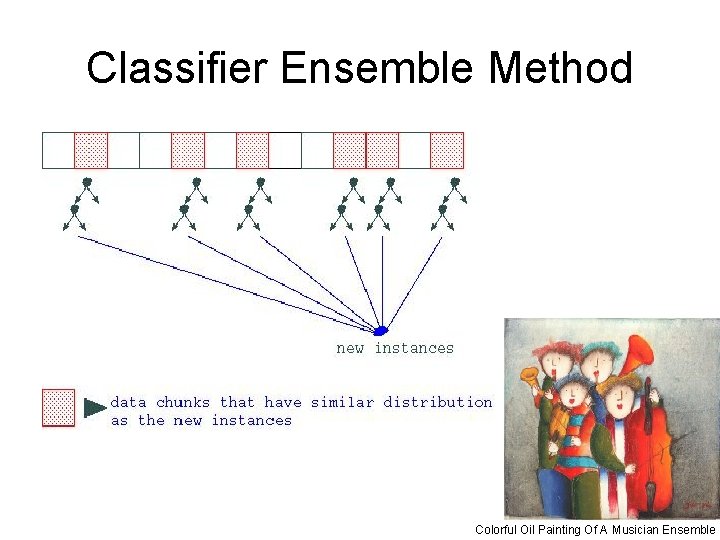
Classifier Ensemble Method Colorful Oil Painting Of A Musician Ensemble

Basic Idea • Steam data is partitioned into sequential chunks • Train a weighted classifier from each chunk • The weight is based on the expected prediction accuracy on the current test examples • Only top K classifiers are kept

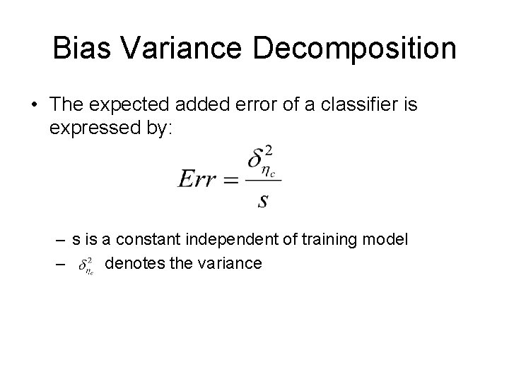
Bias Variance Decomposition • The expected added error of a classifier is expressed by: – s is a constant independent of training model – denotes the variance

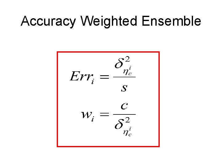
Accuracy Weighted Ensemble

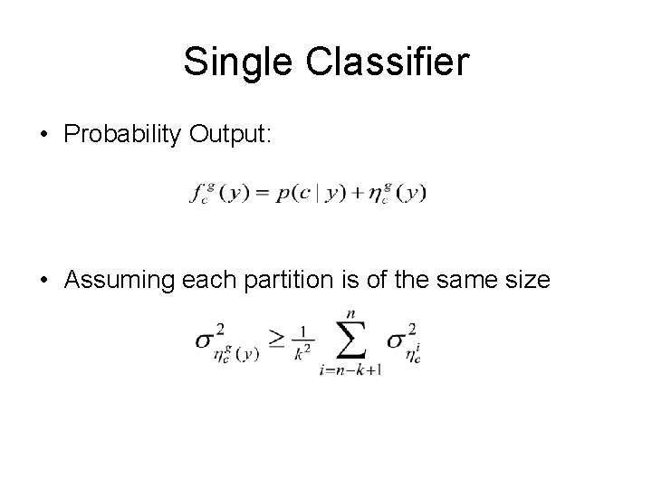
Single Classifier • Probability Output: • Assuming each partition is of the same size

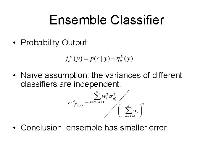
Ensemble Classifier • Probability Output: • Naïve assumption: the variances of different classifiers are independent. • Conclusion: ensemble has smaller error

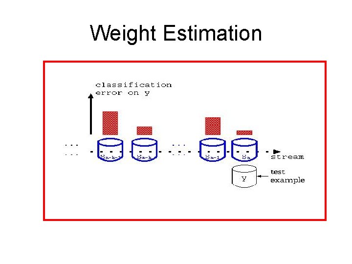
But in reality … • We do not know – Error or variance or the function being learned • Solution: – Use estimation! – Apply the i-th classifier on the current training data to estimate the error of the classifier

Weight Estimation

Problem I: Learning cost is still high • Tree construction has super-linear complexity – Much effort has been made to build a decision tree faster (CLOUD, Rainforest, etc. ) • Approximate methods: Hoeffding bound – We still need to evaluate G() – Incremental updating a non-stable structure • Learn/update a model is costly

Do we care about the shape of the tree? • The Hoeffding method tries to build decision trees “nearly identical” to trees that a batch classifier (ID 3, C 4. 5, Sprint) would build • But batch learner builds decision trees in a divide-and-conquer greedy manner (not optimal anyway)

How about using Random Trees? • Build an ensemble of N random trees • At each node, randomly choose an attribute to split • Throw samples into each tree • Use class label distribution in the leaf nodes as probability output • Constant cost of tree construction • Maximize structural diversity in N trees

Problem II: dependence on the last window • Incrementally maintain a single classifier – tracking patterns in the recent window – the recent window contains the sole training data • Maintain a set of classifiers (an ensemble) – each trained from historical data – Validate classifiers by the most recent data to find “good” classifiers. • There is a flaw: – too much dependence on the most recent data

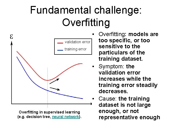
Fundamental challenge: Overfitting validation error training error Overfitting in supervised learning (e. g. decision tree, neural network). • Overfitting: models are too specific, or too sensitive to the particulars of the training dataset. • Symptom: the validation error increases while the training error steadily decreases. • Cause: the training dataset is not large enough, or not representative enough

Overfitting is prevalent in the streaming environment • Inadequacy of training data. – We must avoid conflicting concepts – Small windows are used • Unrepresentative training data. – Stream data is bursty. – Samples may concentrate in a small region of the sample space.

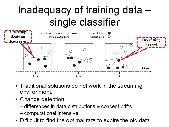
Inadequacy of training data – single classifier Changing decision boundary Overfitting hazard • Traditional solutions do not work in the streaming environment. • Change detection – differences in data distributions concept drifts. – computational intensive • Difficult to find the optimal rate to expire the old data.

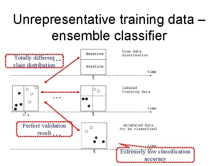
Unrepresentative training data – ensemble classifier Totally different class distribution Perfect validation result Extremely low classification accuracy

How to suppress overfitting in data streams? • For static data, only sample size matters. – enlarging the training dataset to include more instances will help reducing overfitting. • For stream data, we must consider 3 factors: – Size – Space – Time

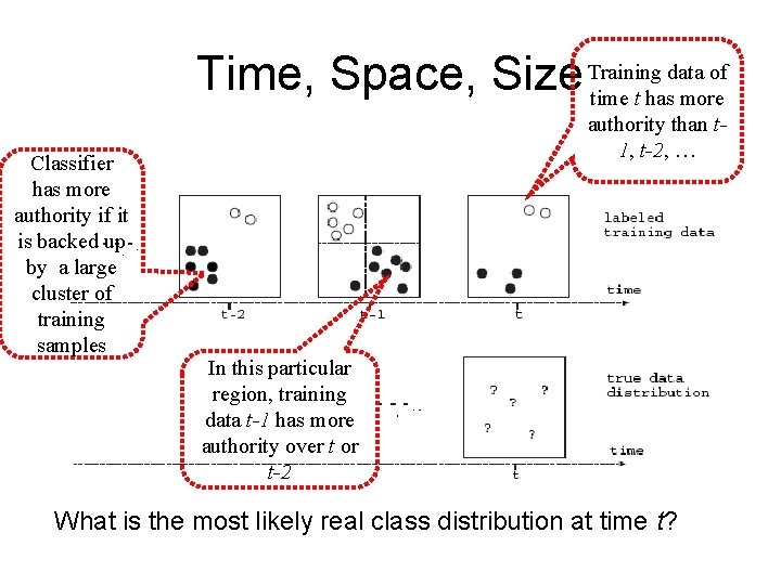
data of Time, Space, Size Training time t has more Classifier has more authority if it is backed up by a large cluster of training samples authority than t 1, t-2, … In this particular region, training data t-1 has more authority over t or t-2 What is the most likely real class distribution at time t?

Summary • To find the most likely current class distribution, consider the time, the space, and the size factors in combining historical classifiers. • How to quantify a historical classifier by time, space, and size? • We formulate the problem from an optimization viewpoint.

Modeling • Distribution changes can occur abruptly – Previous work models smooth, continuous changes • At any given time, the underlying data generating mechanism is in one of multiple states – Within each state, class distribution is stable • State changes are modeled by a Markov model – The aggregated ingress rate is

Modeling • We partition the stream into a sequence of time windows – Time-based windows make more sense than count-based windows for concept drifts • We partition the feature space V into a set of non-overlapping regions. – Bursty arrivals may concentrate in one region. • Weight classifiers by time and region.

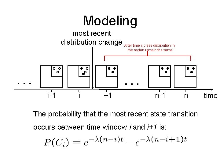
Modeling most recent distribution change After time i, class distribution in the region remain the same … … i-1 i i+1 n-1 n The probability that the most recent state transition occurs between time window i and i+1 is: time

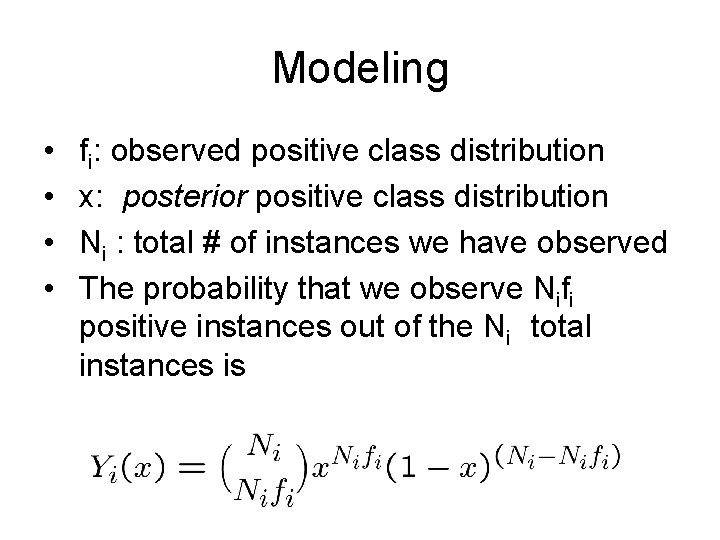
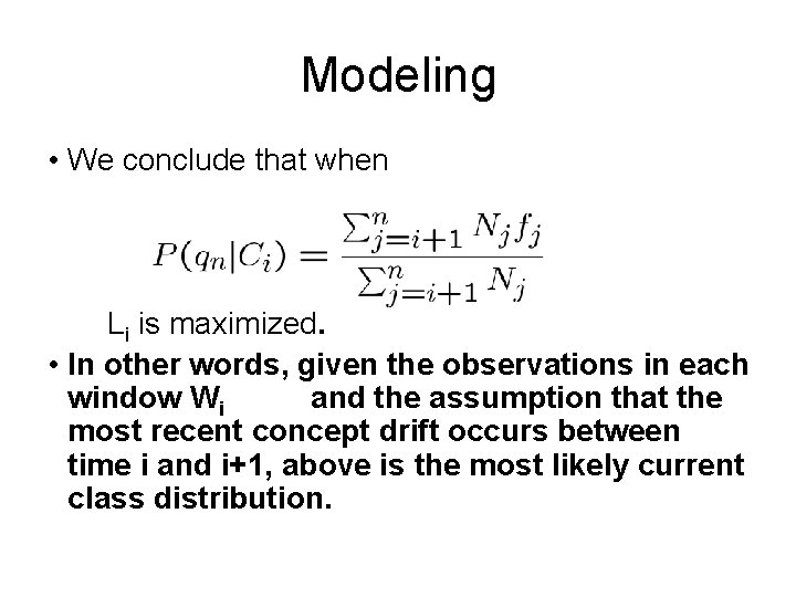
Modeling • • fi: observed positive class distribution x: posterior positive class distribution Ni : total # of instances we have observed The probability that we observe Nifi positive instances out of the Ni total instances is

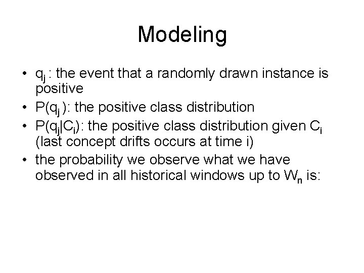
Modeling • qj : the event that a randomly drawn instance is positive • P(qj ): the positive class distribution • P(qj|Ci): the positive class distribution given Ci (last concept drifts occurs at time i) • the probability we observe what we have observed in all historical windows up to Wn is:

Modeling • We conclude that when Li is maximized. • In other words, given the observations in each window Wi and the assumption that the most recent concept drift occurs between time i and i+1, above is the most likely current class distribution.

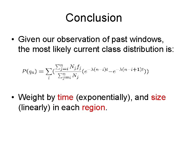
Conclusion • Given our observation of past windows, the most likely current class distribution is: • Weight by time (exponentially), and size (linearly) in each region.

Summary • To handle concept drifts – we keep on learning new models – we keep throwing away old models – the data we rely on is a tiny portion of the infinite stream

But history always repeats itself • Assumption: the data generation mechanism works in different states • In each state, the class distribution is stable • State transition can occur anytime • The total number of states are limited

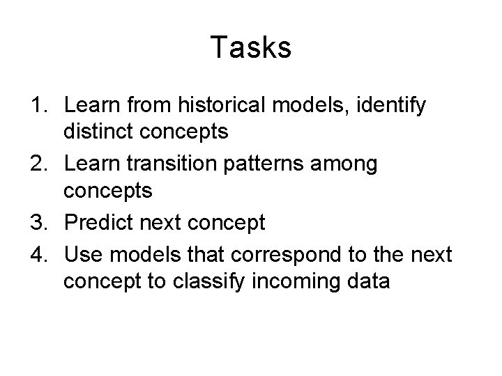
Tasks 1. Learn from historical models, identify distinct concepts 2. Learn transition patterns among concepts 3. Predict next concept 4. Use models that correspond to the next concept to classify incoming data

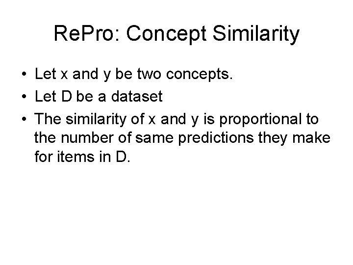
Re. Pro [KDD’ 05] • Trigger – Using a current model, and monitor whether accumulated error exceeds a threshold • Finding a concept – If error > threshold, learn a new concept c – Compare c with historical concepts xi – If similarity between c and any xi is less than a threshold, add c into historical concepts • Transition matrix – A first order Markov chain of concepts

Re. Pro: Concept Similarity • Let x and y be two concepts. • Let D be a dataset • The similarity of x and y is proportional to the number of same predictions they make for items in D.

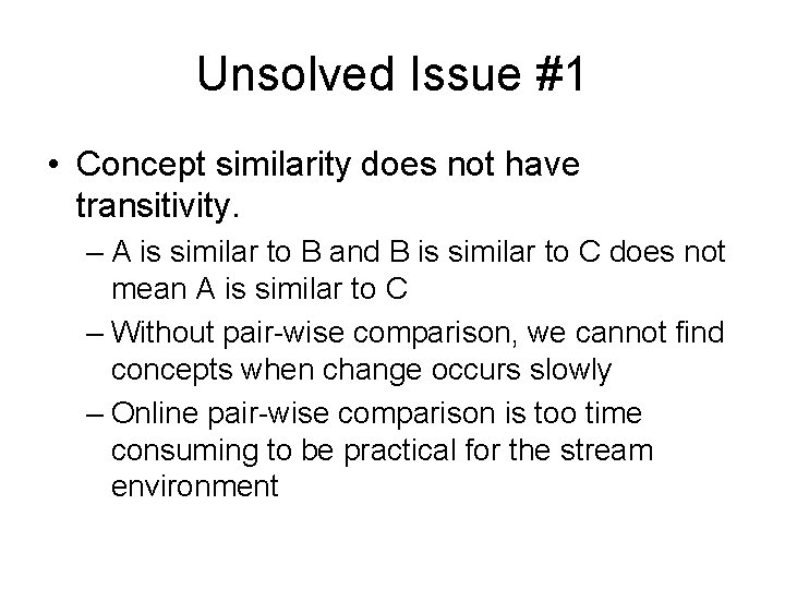
Unsolved Issue #1 • Concept similarity does not have transitivity. – A is similar to B and B is similar to C does not mean A is similar to C – Without pair-wise comparison, we cannot find concepts when change occurs slowly – Online pair-wise comparison is too time consuming to be practical for the stream environment

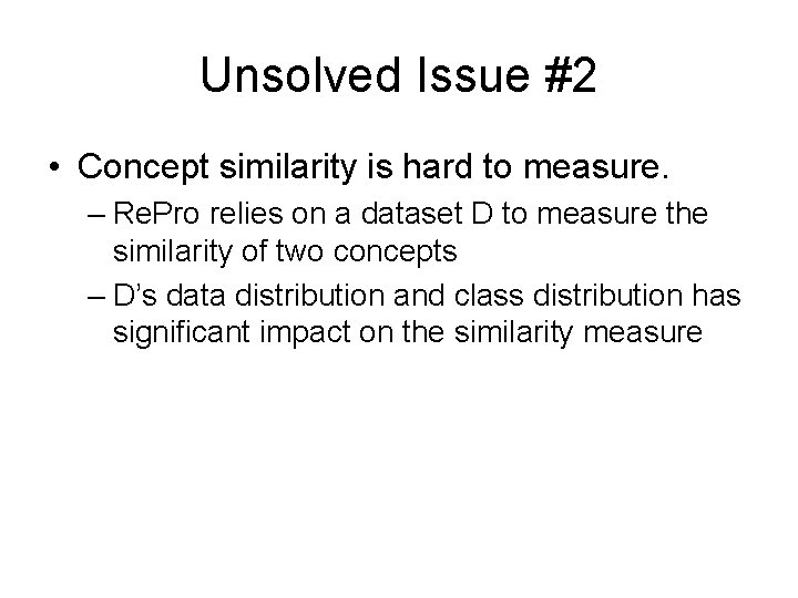
Unsolved Issue #2 • Concept similarity is hard to measure. – Re. Pro relies on a dataset D to measure the similarity of two concepts – D’s data distribution and class distribution has significant impact on the similarity measure

Unsolved Issue #3 • Re. Pro is heavily dependent on parameters – The stable threshold – The trigger threshold – The concept similarity threshold

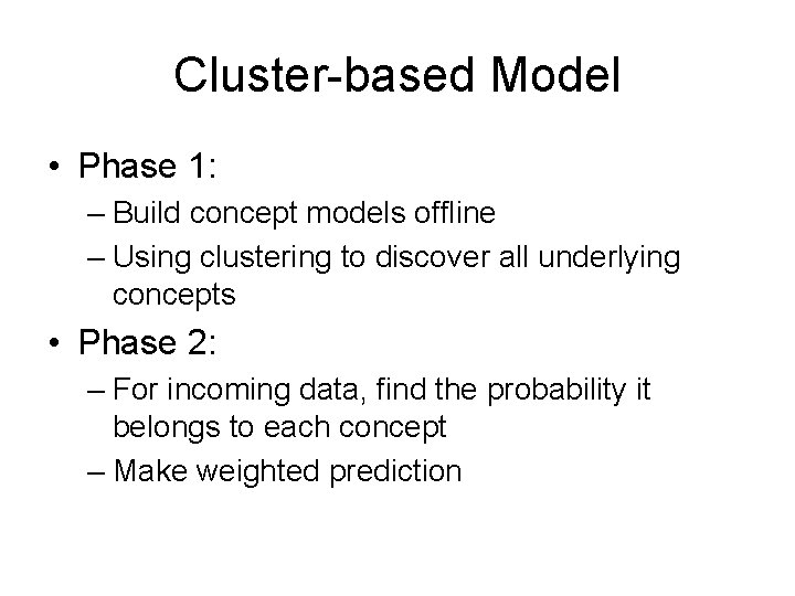
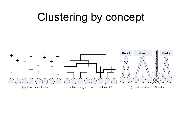
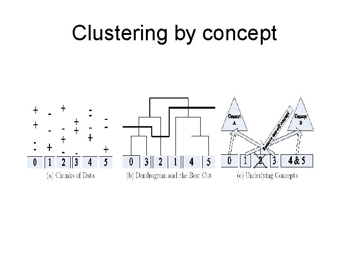
Cluster-based Model • Phase 1: – Build concept models offline – Using clustering to discover all underlying concepts • Phase 2: – For incoming data, find the probability it belongs to each concept – Make weighted prediction

Clustering by concept

Clustering by concept

PART II Applying Classifiers on Streams Issues: Accuracy, Cost (CPU, bandwidth, …), Load Shedding

Background: Load Shedding • Load shedding — dropping certain data when the system is overloaded. • Current studies on load shedding focus on answering traditional (aggregation) queries, not on mining data streams. • Cost is a major concern in classifying data streams – E. g. a large number of sensors simultaneously send data to central server for real time analysis – Central server cannot afford enough bandwidth and CPU resource to handle them

Optimization Problem • Resource allocation as optimization problems: – minimizes resource usage subjective to a lower bound on precision – maximizes the precision subjective to an upper bound on resource

Possible Solutions • Randomly shedding load – degradation of classification quality • Using user-provided Qo. S metrics to shed load – Qo. S metric is often unavailable in dynamically changing stream environment

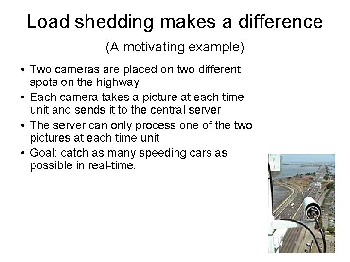
Load shedding makes a difference (A motivating example) • Two cameras are placed on two different spots on the highway • Each camera takes a picture at each time unit and sends it to the central server • The server can only process one of the two pictures at each time unit • Goal: catch as many speeding cars as possible in real-time.

Load shedding makes a difference (A motivating example) • Assumptions: – At any time, highway A contains a speeding car with probability p. A; highway B contains a speeding car with probability p. B – p. A and p. B change with time – The classifier is always accurate

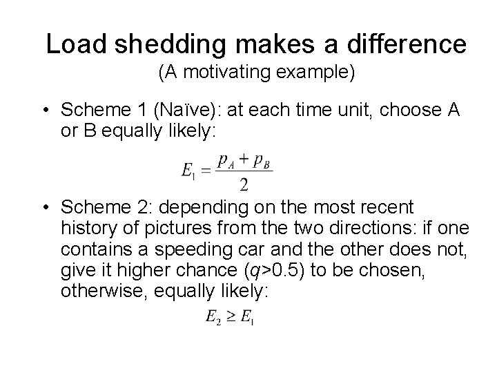
Load shedding makes a difference (A motivating example) • Scheme 1 (Naïve): at each time unit, choose A or B equally likely: • Scheme 2: depending on the most recent history of pictures from the two directions: if one contains a speeding car and the other does not, give it higher chance (q>0. 5) to be chosen, otherwise, equally likely:

Load shedding makes a difference (A motivating example) • Scheme 2 automatically focuses on data with higher benefits; • Scheme 2 does not depends on the parameters p. A and p. B, so if they drift with time, the scheme can adapt to the new parameters automatically.

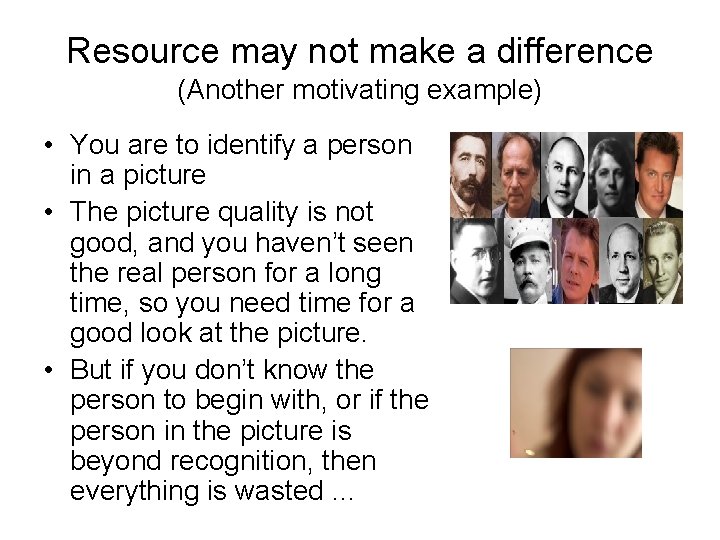
Resource may not make a difference (Another motivating example) • You are to identify a person in a picture • The picture quality is not good, and you haven’t seen the real person for a long time, so you need time for a good look at the picture. • But if you don’t know the person to begin with, or if the person in the picture is beyond recognition, then everything is wasted …

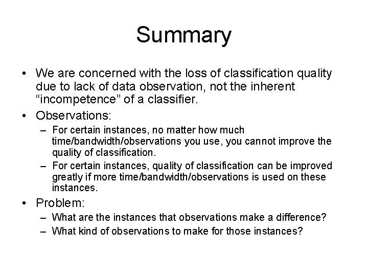
Summary • We are concerned with the loss of classification quality due to lack of data observation, not the inherent “incompetence” of a classifier. • Observations: – For certain instances, no matter how much time/bandwidth/observations you use, you cannot improve the quality of classification. – For certain instances, quality of classification can be improved greatly if more time/bandwidth/observations is used on these instances. • Problem: – What are the instances that observations make a difference? – What kind of observations to make for those instances?

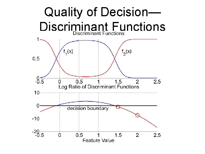
Load. Star [SDM 2004] • A Quality of Decision (Qo. D) measure – If Qo. D is high, then we don’t want to spend more time on the input: the current classification is already good. – If Qo. D is low, then we should give the classifier more resource so that it can make a better decision • Qo. D is based on the prediction of feature value at the next time unit

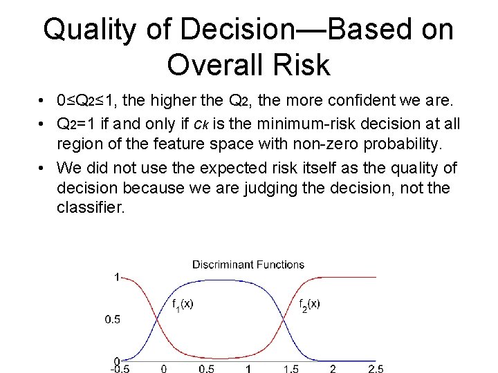
Quality of Decision— Discriminant Functions

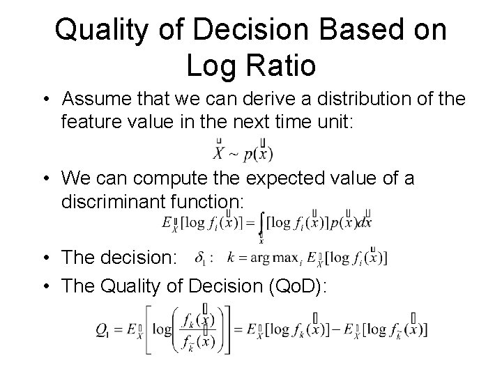
Quality of Decision Based on Log Ratio • Assume that we can derive a distribution of the feature value in the next time unit: • We can compute the expected value of a discriminant function: • The decision: • The Quality of Decision (Qo. D):

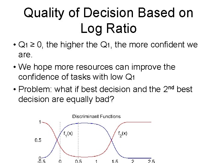
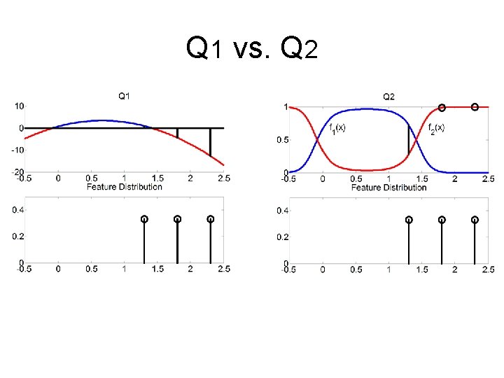
Quality of Decision Based on Log Ratio • Q 1 ≥ 0, the higher the Q 1, the more confident we are. • We hope more resources can improve the confidence of tasks with low Q 1 • Problem: what if best decision and the 2 nd best decision are equally bad?

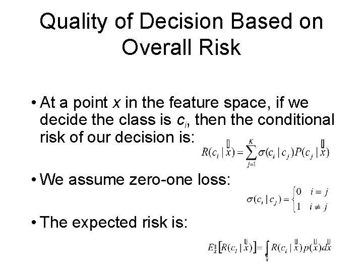
Quality of Decision Based on Overall Risk • At a point x in the feature space, if we decide the class is ci, then the conditional risk of our decision is: • We assume zero-one loss: • The expected risk is:

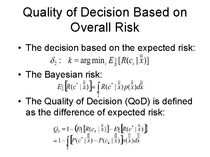
Quality of Decision Based on Overall Risk • The decision based on the expected risk: • The Bayesian risk: • The Quality of Decision (Qo. D) is defined as the difference of expected risk:

Quality of Decision—Based on Overall Risk • 0≤Q 2≤ 1, the higher the Q 2, the more confident we are. • Q 2=1 if and only if ck is the minimum-risk decision at all region of the feature space with non-zero probability. • We did not use the expected risk itself as the quality of decision because we are judging the decision, not the classifier.

Q 1 vs. Q 2

Quality of Decision—Naïve Bayesian Classifier • By “naïve”, we assume that the distributions of the feature values are conditionally independent given the class labels; • By “Bayesian”, we restrict our discriminant functions to be the posterior distributions of each class. • It has been shown that the performance of naïve Bayesian classifiers are competitive with other sophisticated classifiers. • The computation is simplified with the assumption of conditional independence.

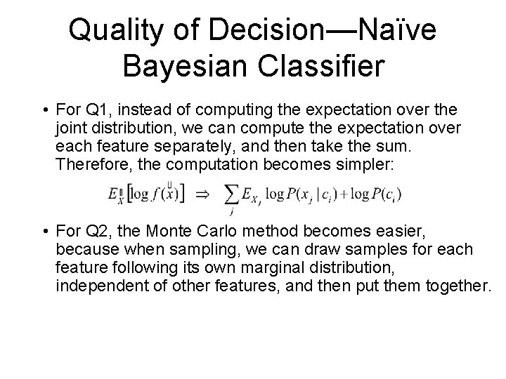
Quality of Decision—Naïve Bayesian Classifier • For Q 1, instead of computing the expectation over the joint distribution, we can compute the expectation over each feature separately, and then take the sum. Therefore, the computation becomes simpler: • For Q 2, the Monte Carlo method becomes easier, because when sampling, we can draw samples for each feature following its own marginal distribution, independent of other features, and then put them together.

Feature Prediction—Challenges • The feature distribution in the next time unit: • We can simply use the prior distribution. • However, we can do better—taking advantage of temporal locality: – sensors that measure temperature or river water level – images of consecutive snapshots from satellite • In addition, the data characteristics may drift with time —time-varying models.

Movement prediction • To make intelligent load shedding decisions at time t, we need to know the distribution of a point’s position at time t+1. • Our assumption: – a point’s location in the feature space at time t+1 solely depends on its location at time t. – features are independent to each other with regard to points’ movement • We build a Markov model for each feature

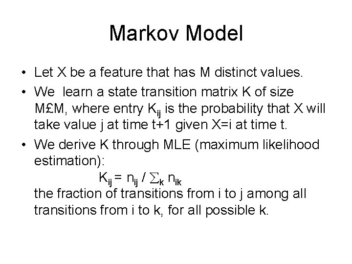
Markov Model • Let X be a feature that has M distinct values. • We learn a state transition matrix K of size M£M, where entry Kij is the probability that X will take value j at time t+1 given X=i at time t. • We derive K through MLE (maximum likelihood estimation): Kij = nij / k nik the fraction of transitions from i to j among all transitions from i to k, for all possible k.

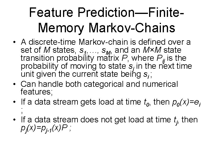
Feature Prediction—Finite. Memory Markov-Chains • A discrete-time Markov-chain is defined over a set of M states, s 1, …, s. M, and an M×M state transition probability matrix P, where Pij is the probability of moving to state sj in the next time unit given the current state being si ; • Can handle both categorical and numerical features; • If a data stream gets load at time t 0, then p 0(x)=ei ; • If a data stream does not get load at time tj, then pj(x)=pj-1(x)P ;

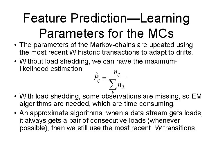
Feature Prediction—Learning Parameters for the MCs • The parameters of the Markov-chains are updated using the most recent W historic transactions to adapt to drifts. • Without load shedding, we can have the maximumlikelihood estimation: • With load shedding, some observations are missing, so EM algorithms are needed, which are time consuming. • An approximate algorithms: when a data stream gets loads, it always gets a pair of consecutive loads (whenever possible), then we still use the most recent W transitions.

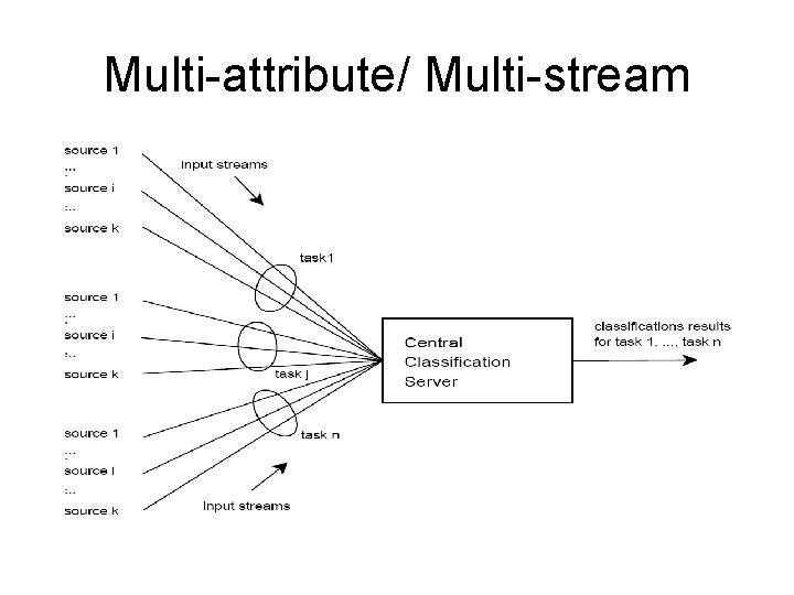
Multi-attribute/ Multi-stream

Problem • A central classifier – monitors n×k streams from n tasks, – has capacity to process m out of the n×k input streams. • which of the input streams should be inspected so that the classification quality is least affected?

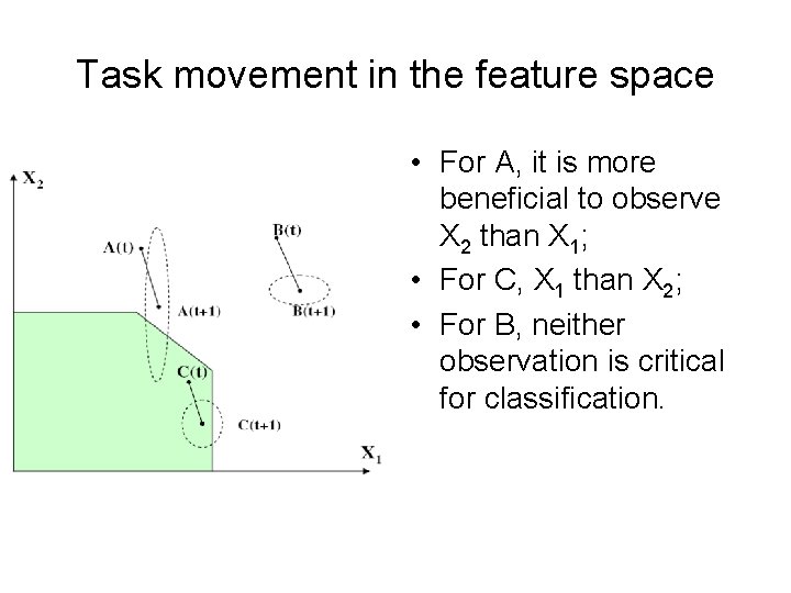
Task movement in the feature space • For A, it is more beneficial to observe X 2 than X 1; • For C, X 1 than X 2; • For B, neither observation is critical for classification.

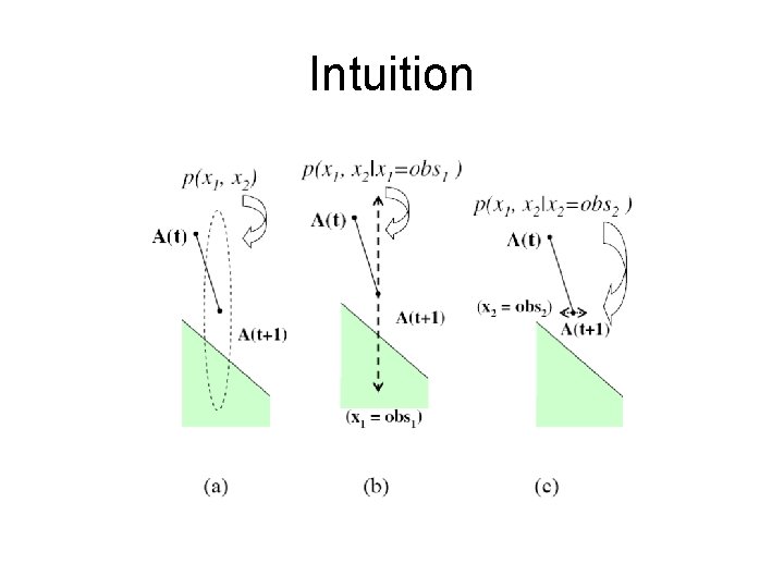
Intuition

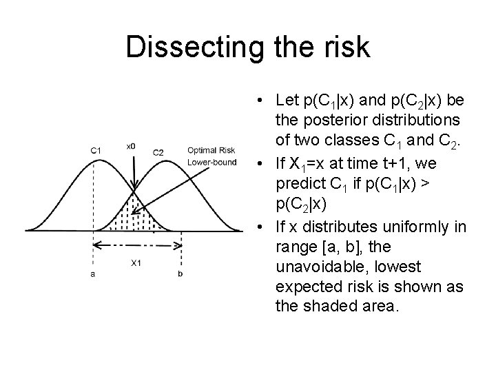
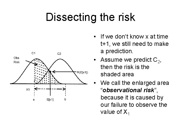
Dissecting the risk • Let p(C 1|x) and p(C 2|x) be the posterior distributions of two classes C 1 and C 2. • If X 1=x at time t+1, we predict C 1 if p(C 1|x) > p(C 2|x) • If x distributes uniformly in range [a, b], the unavoidable, lowest expected risk is shown as the shaded area.

Dissecting the risk • If we don’t know x at time t+1, we still need to make a prediction. • Assume we predict C 2, then the risk is the shaded area • We call the enlarged area “observational risk”, because it is caused by our failure to observe the value of X 1

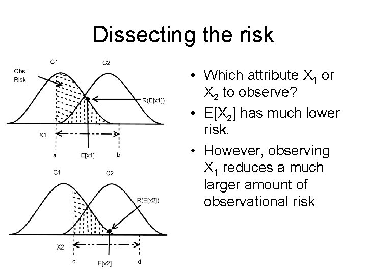
Dissecting the risk • Which attribute X 1 or X 2 to observe? • E[X 2] has much lower risk. • However, observing X 1 reduces a much larger amount of observational risk

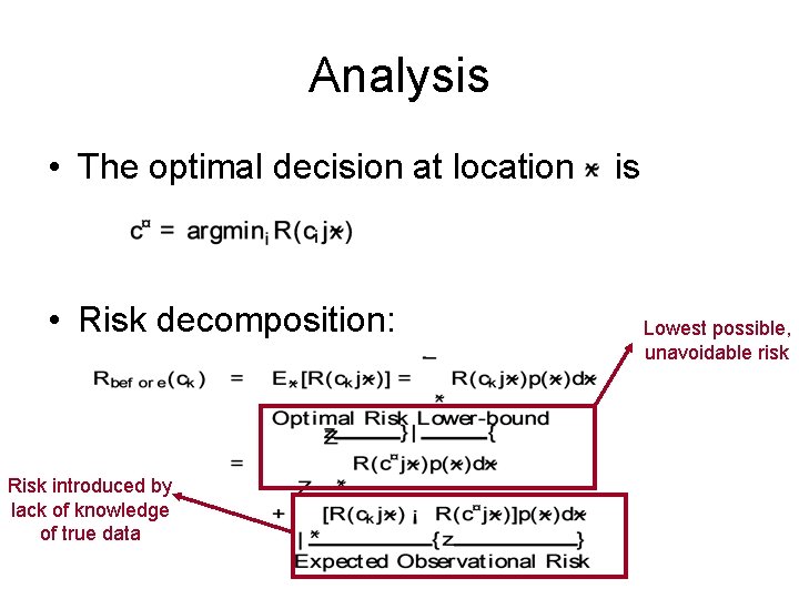
Analysis • The optimal decision at location • Risk decomposition: Risk introduced by lack of knowledge of true data is Lowest possible, unavoidable risk

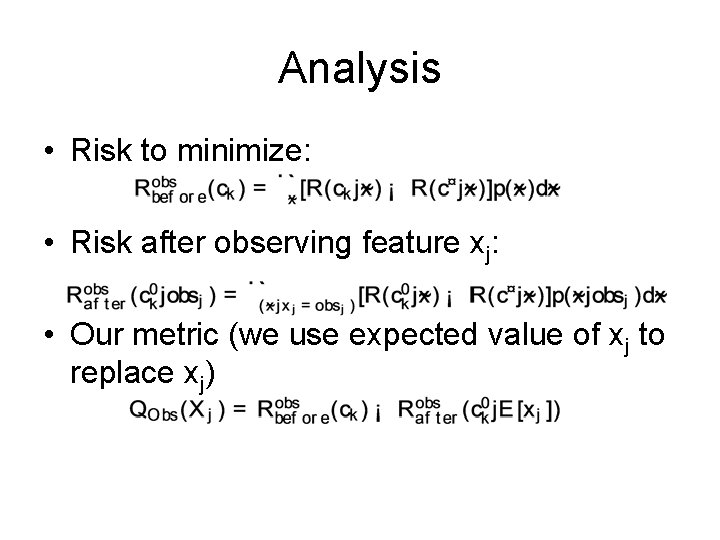
Analysis • Risk to minimize: • Risk after observing feature xj: • Our metric (we use expected value of xj to replace xj)

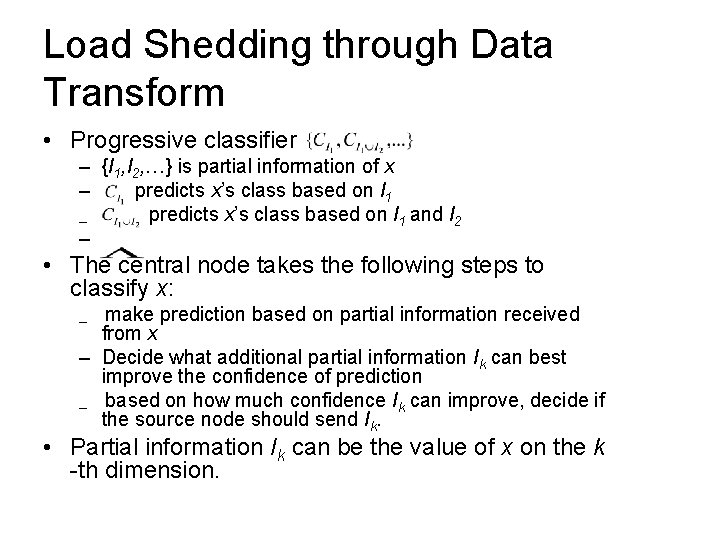
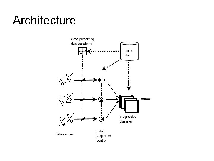
Load Shedding through Data Transform • Progressive classifier – {I 1, I 2, …} is partial information of x – predicts x’s class based on I 1 and I 2 – – • The central node takes the following steps to classify x: make prediction based on partial information received from x – Decide what additional partial information Ik can best improve the confidence of prediction – based on how much confidence Ik can improve, decide if the source node should send Ik. – • Partial information Ik can be the value of x on the k -th dimension.

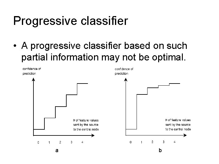
Progressive classifier • A progressive classifier based on such partial information may not be optimal. a b

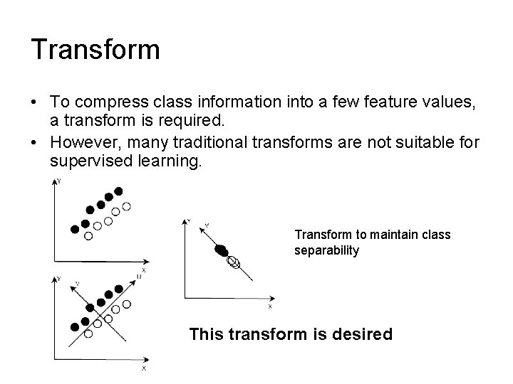
Progressive classifier • We want to design a progressive classifier which has the following properties: – The “class information” concentrates on the first few features – The features are independent of each other • Prevents a classifier from inspecting a feature whose “class information” is covered by features already inspected

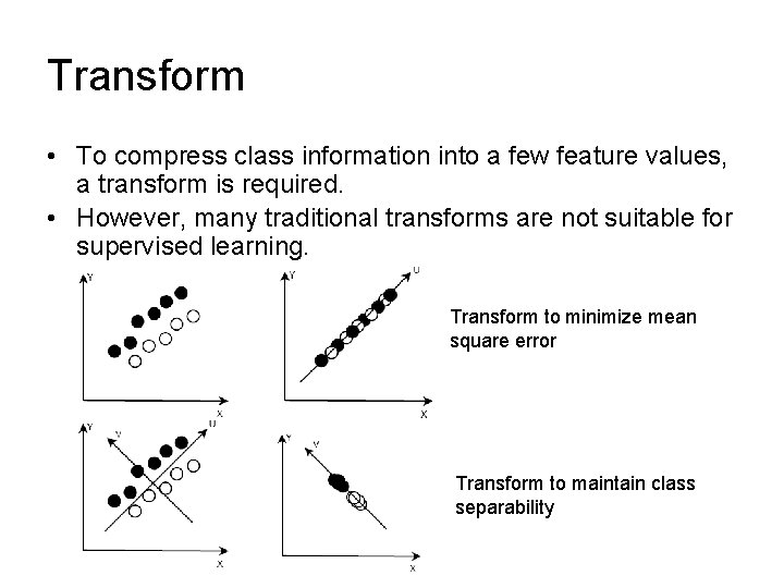
Transform • To compress class information into a few feature values, a transform is required. • However, many traditional transforms are not suitable for supervised learning. Transform to minimize mean square error Transform to maintain class separability

Transform • To compress class information into a few feature values, a transform is required. • However, many traditional transforms are not suitable for supervised learning. Transform to maintain class separability This transform is desired

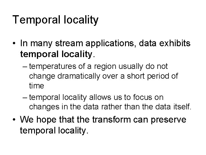
Temporal locality • In many stream applications, data exhibits temporal locality. – temperatures of a region usually do not change dramatically over a short period of time – temporal locality allows us to focus on changes in the data rather than the data itself. • We hope that the transform can preserve temporal locality.

Architecture

Conclusion • Classification is a most important task on stream data analysis • Data volume and change of data distribution pose challenges to learning models and using models • Intelligent model reusing and intelligent load shedding are good solutions

Fair Use Agreement This agreement covers the use of all slides on this CD-Rom, please read carefully. • You may freely use these slides for teaching, if • You send me an email telling me the class number/ university in advance. • My name and email address appears on the first slide (if you are using all or most of the slides), or on each slide (if you are just taking a few slides). • You may freely use these slides for a conference presentation, if • You send me an email telling me the conference name in advance. • My name appears on each slide you use. • You may not use these slides for tutorials, or in a published work (tech report/ conference paper/ thesis/ journal etc). If you wish to do this, email me first, it is highly likely I will grant you permission. (c) Haixun Wang, haixun@us. ibm. com