Introduction to Phylogenetic Estimation Algorithms Tandy Warnow Phylogeny

Introduction to Phylogenetic Estimation Algorithms Tandy Warnow

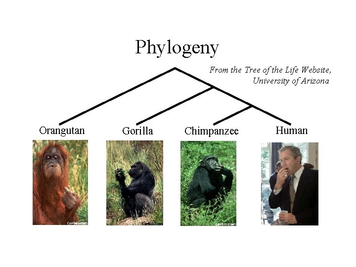
Phylogeny From the Tree of the Life Website, University of Arizona Orangutan Gorilla Chimpanzee Human

Phylogenetic Analysis • • Gather data Align sequences Estimate phylogeny on the multiple alignment Estimate the reliable aspects of the evolutionary history (using bootstrapping, consensus trees, or other methods) • Perform post-tree analyses

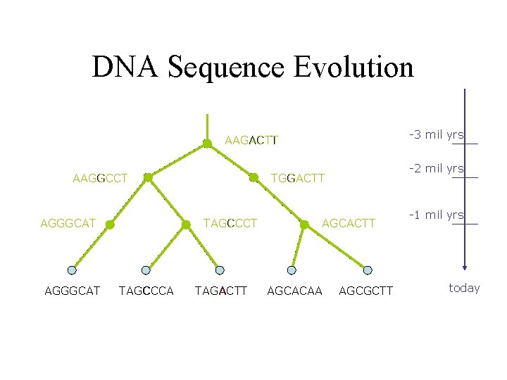
DNA Sequence Evolution -3 mil yrs AAGACTT AAGGCCT AGGGCAT TAGCCCA -2 mil yrs TGGACTT TAGACTT AGCACAA AGCGCTT -1 mil yrs today

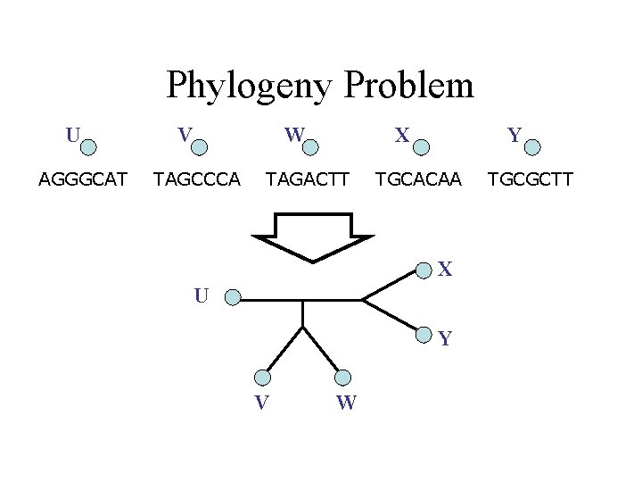
Phylogeny Problem U AGGGCAT V W TAGCCCA X TAGACTT Y TGCACAA X U Y V W TGCGCTT

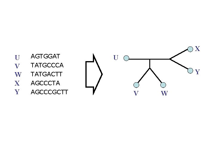
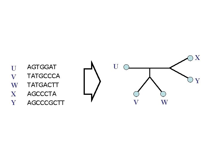
X U V W X Y AGTGGAT TATGCCCA TATGACTT AGCCCTA AGCCCGCTT U Y V W

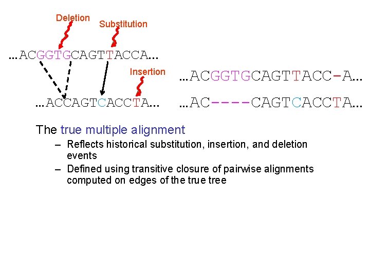
Deletion Substitution …ACGGTGCAGTTACCA… Insertion …ACCAGTCACCTA… …ACGGTGCAGTTACC-A… …AC----CAGTCACCTA… The true multiple alignment – Reflects historical substitution, insertion, and deletion events – Defined using transitive closure of pairwise alignments computed on edges of the true tree

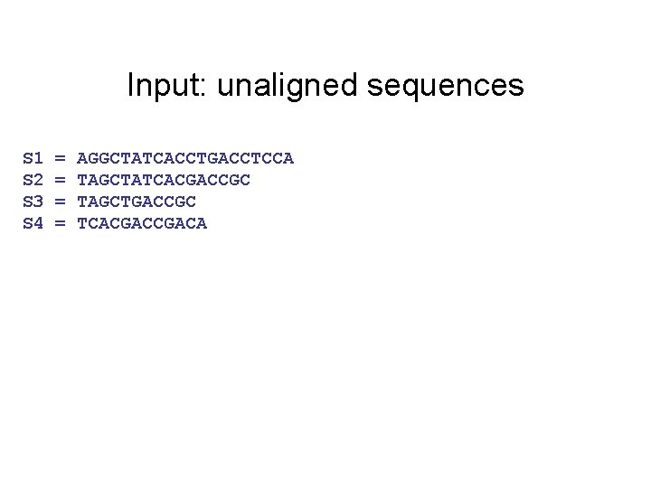
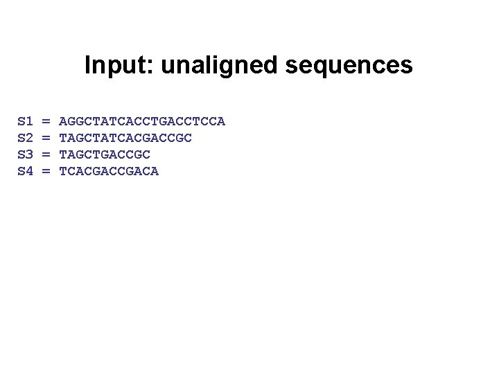
Input: unaligned sequences S 1 S 2 S 3 S 4 = = AGGCTATCACCTGACCTCCA TAGCTATCACGACCGC TAGCTGACCGC TCACGACA

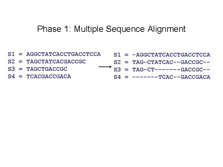
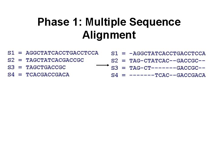
Phase 1: Multiple Sequence Alignment S 1 S 2 S 3 S 4 = = AGGCTATCACCTGACCTCCA TAGCTATCACGACCGC TAGCTGACCGC TCACGACA S 1 S 2 S 3 S 4 = = -AGGCTATCACCTGACCTCCA TAG-CTATCAC--GACCGC-TAG-CT-------GACCGC----TCAC--GACCGACA

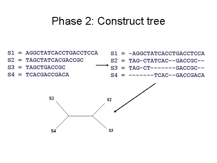
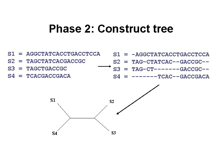
Phase 2: Construct tree S 1 S 2 S 3 S 4 = = AGGCTATCACCTGACCTCCA TAGCTATCACGACCGC TAGCTGACCGC TCACGACA S 1 S 4 S 1 S 2 S 3 S 4 S 2 S 3 = = -AGGCTATCACCTGACCTCCA TAG-CTATCAC--GACCGC-TAG-CT-------GACCGC----TCAC--GACCGACA

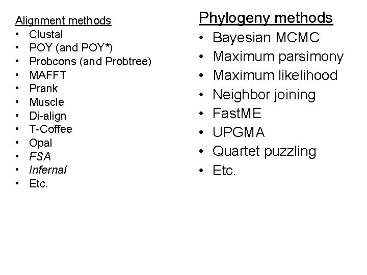
Alignment methods • Clustal • POY (and POY*) • Probcons (and Probtree) • MAFFT • Prank • Muscle • Di-align • T-Coffee • Opal • FSA • Infernal • Etc. Phylogeny methods • • Bayesian MCMC Maximum parsimony Maximum likelihood Neighbor joining Fast. ME UPGMA Quartet puzzling Etc. RAx. ML: best heuristic for large-scale ML optimization

• How are methods evaluated? • Which methods perform well? • What about other evolutionary processes, such as duplications or rearrangements? • What if the phylogeny is not a tree? • What are the major outstanding challenges?

• Part I (Basics): standard statistical models of substitution-only sequence evolution, methods for phylogeny estimation, performance criteria, and basic proof techniques. • Part II (Advanced): Alignment estimation, more complex models of sequence evolution, species tree estimation from gene trees and sequences, reticulate evolution, and gene order/content phylogeny.

Part I: Basics • • • Substitution-only models of evolution Performance criteria Standard methods for phylogeny estimation Statistical performance guarantees and proof techniques Performance on simulated and real data Evaluating support

DNA Sequence Evolution -3 mil yrs AAGACTT AAGGCCT AGGGCAT TAGCCCA -2 mil yrs TGGACTT TAGACTT AGCACAA AGCGCTT -1 mil yrs today

Phylogeny Problem U AGGGCAT V W TAGCCCA X TAGACTT Y TGCACAA X U Y V W TGCGCTT

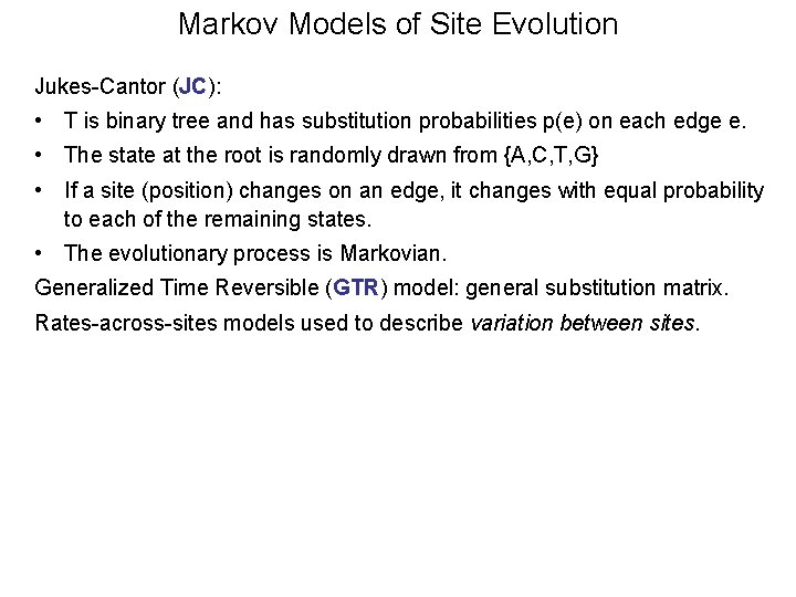
Markov Models of Site Evolution Jukes-Cantor (JC): • T is binary tree and has substitution probabilities p(e) on each edge e. • The state at the root is randomly drawn from {A, C, T, G} • If a site (position) changes on an edge, it changes with equal probability to each of the remaining states. • The evolutionary process is Markovian. Generalized Time Reversible (GTR) model: general substitution matrix. Rates-across-sites models used to describe variation between sites.

Performance criteria • Running time and space. • Statistical performance issues (e. g. , statistical consistency and sequence length requirements), typically studied mathematically. • “Topological accuracy” with respect to the underlying true tree. Typically studied in simulation. • Accuracy with respect to a mathematical score (e. g. tree length or likelihood score) on real data.

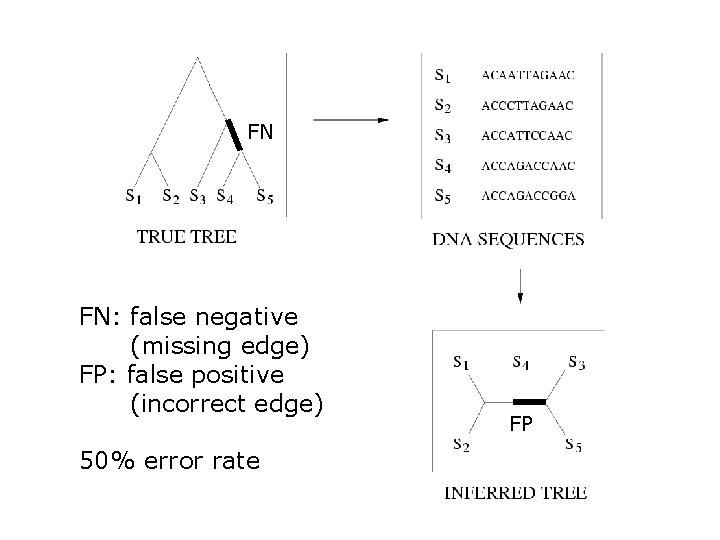
FN FN: false negative (missing edge) FP: false positive (incorrect edge) 50% error rate FP

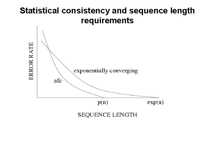
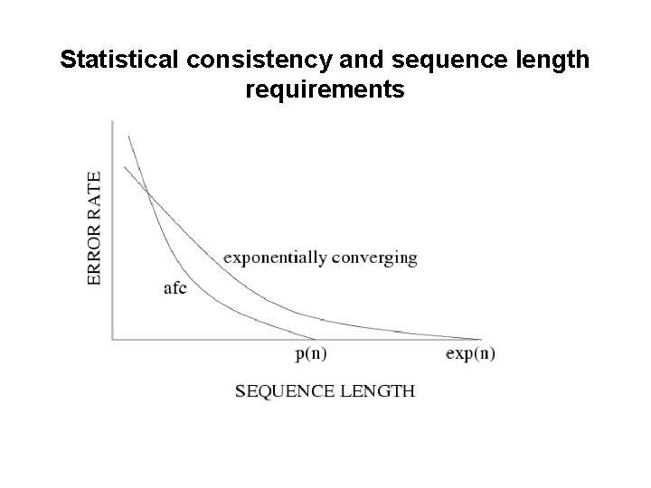
Statistical consistency and sequence length requirements

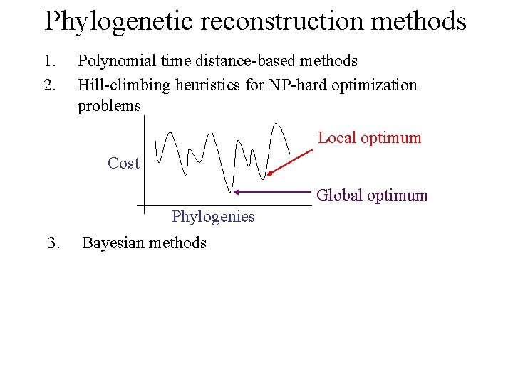
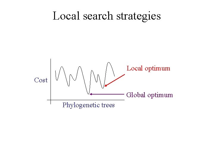
Phylogenetic reconstruction methods 1. 2. Polynomial time distance-based methods Hill-climbing heuristics for NP-hard optimization problems Local optimum Cost Global optimum Phylogenies 3. Bayesian methods

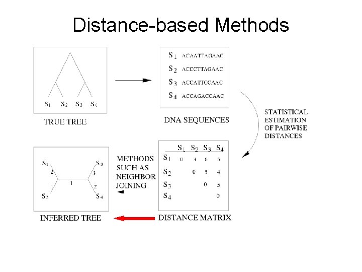
Distance-based Methods

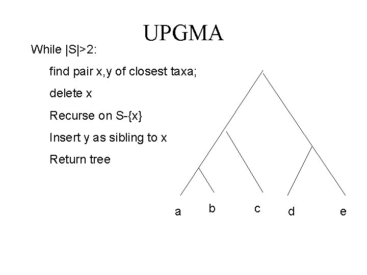
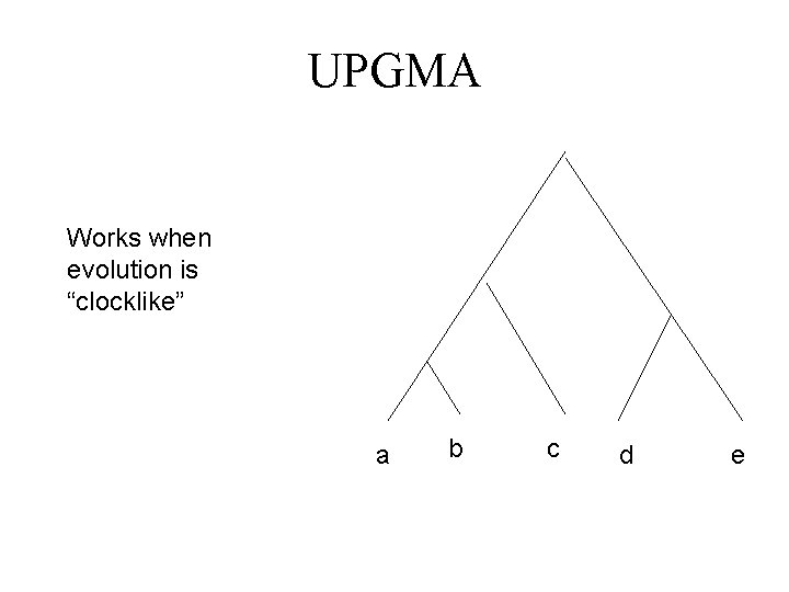
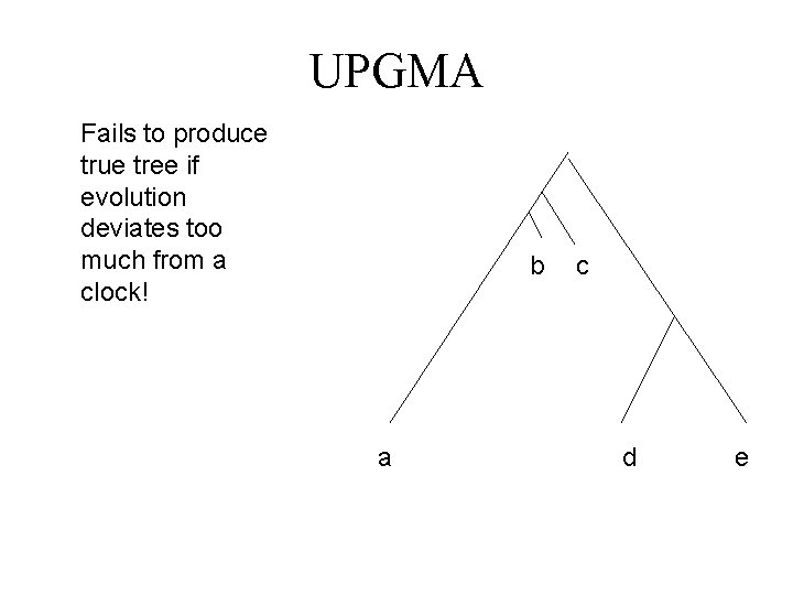
While |S|>2: UPGMA find pair x, y of closest taxa; delete x Recurse on S-{x} Insert y as sibling to x Return tree a b c d e

UPGMA Works when evolution is “clocklike” a b c d e

UPGMA Fails to produce true tree if evolution deviates too much from a clock! b a c d e

Distance-based Methods

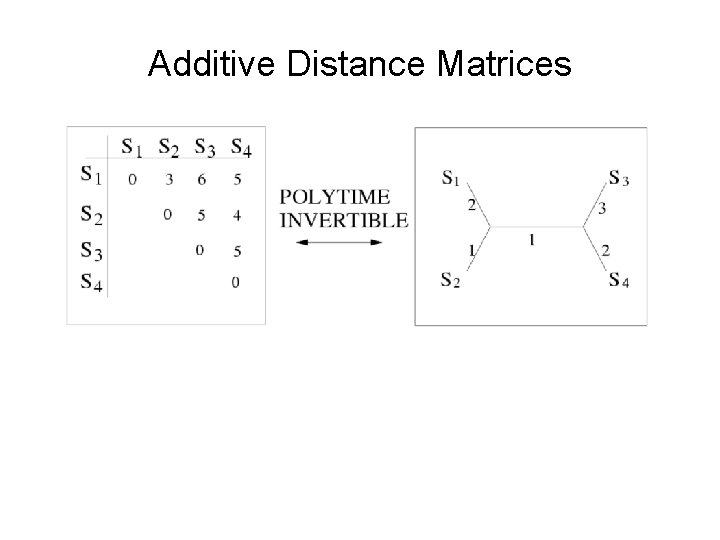
Additive Distance Matrices

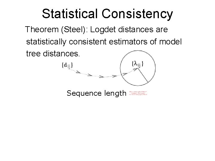
Statistical Consistency Theorem (Steel): Logdet distances are statistically consistent estimators of model tree distances. Sequence length

Distance-based Methods

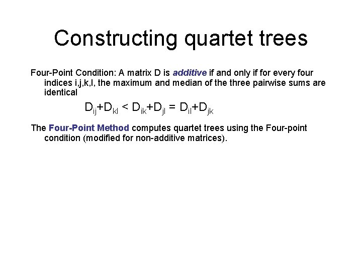
Constructing quartet trees Four-Point Condition: A matrix D is additive if and only if for every four indices i, j, k, l, the maximum and median of the three pairwise sums are identical Dij+Dkl < Dik+Djl = Dil+Djk The Four-Point Method computes quartet trees using the Four-point condition (modified for non-additive matrices).

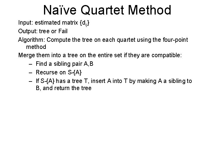
Naïve Quartet Method Input: estimated matrix {dij} Output: tree or Fail Algorithm: Compute the tree on each quartet using the four-point method Merge them into a tree on the entire set if they are compatible: – Find a sibling pair A, B – Recurse on S-{A} – If S-{A} has a tree T, insert A into T by making A a sibling to B, and return the tree

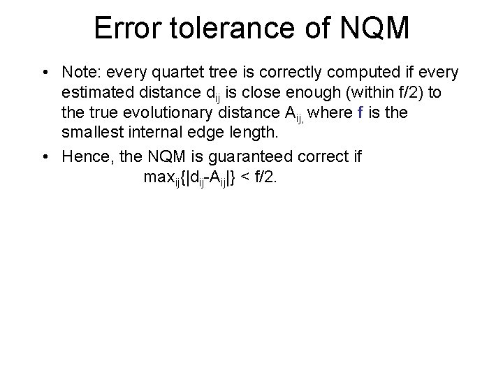
Error tolerance of NQM • Note: every quartet tree is correctly computed if every estimated distance dij is close enough (within f/2) to the true evolutionary distance Aij, where f is the smallest internal edge length. • Hence, the NQM is guaranteed correct if maxij{|dij-Aij|} < f/2.

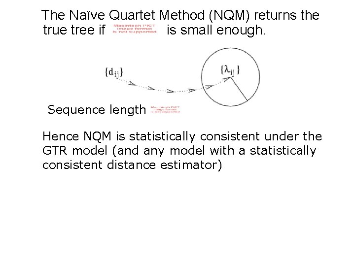
The Naïve Quartet Method (NQM) returns the true tree if is small enough. Sequence length Hence NQM is statistically consistent under the GTR model (and any model with a statistically consistent distance estimator)

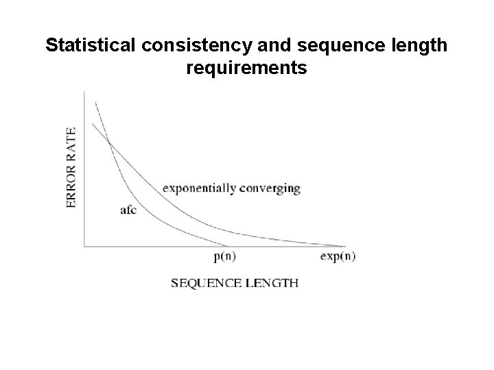
Statistical consistency and sequence length requirements

Theorem (Erdos et al. 1999): The Naïve Quartet Method will return the true tree w. h. p. provided sequence lengths are exponential in the evolutionary diameter of the tree. Sketch of proof: • NQM guaranteed correct if all entries in the estimated distance matrix have low error. • Estimations of large distances require long sequences to have low error with high probability (w. h. p). Note: Other methods have the same guarantee (various authors), and better empirical performance.

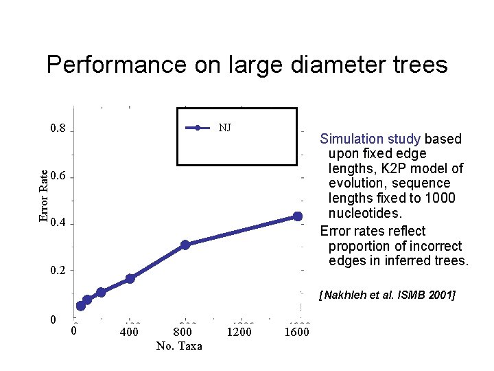
Performance on large diameter trees Error Rate 0. 8 NJ Simulation study based upon fixed edge lengths, K 2 P model of evolution, sequence lengths fixed to 1000 nucleotides. Error rates reflect proportion of incorrect edges in inferred trees. 0. 6 0. 4 0. 2 [Nakhleh et al. ISMB 2001] 0 0 400 800 No. Taxa 1200 1600

Statistical consistency and sequence length requirements

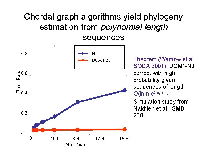
Chordal graph algorithms yield phylogeny estimation from polynomial length sequences Error Rate 0. 8 NJ DCM 1 -NJ • Theorem (Warnow et al. , SODA 2001): DCM 1 -NJ correct with high probability given sequences of length O(ln n e. O(g ln n)) • Simulation study from Nakhleh et al. ISMB 2001 0. 6 0. 4 0. 2 0 0 400 800 No. Taxa 1200 1600

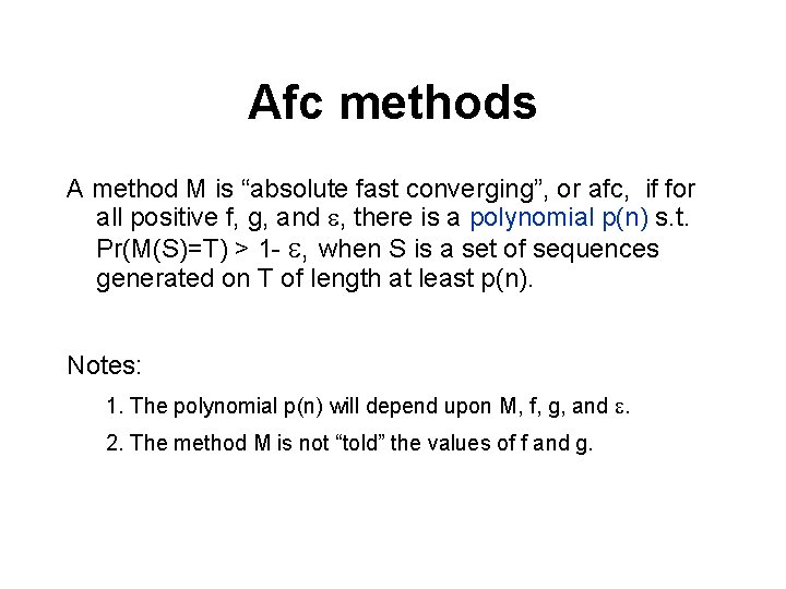
Afc methods A method M is “absolute fast converging”, or afc, if for all positive f, g, and , there is a polynomial p(n) s. t. Pr(M(S)=T) > 1 - , when S is a set of sequences generated on T of length at least p(n). Notes: 1. The polynomial p(n) will depend upon M, f, g, and . 2. The method M is not “told” the values of f and g.

Fast converging methods (and related work) • 1997: Erdos, Steel, Szekely, and Warnow (ICALP). • 1999: Erdos, Steel, Szekely, and Warnow (RSA, TCS); Huson, Nettles and Warnow (J. Comp Bio. ) • 2001: Warnow, St. John, and Moret (SODA); Cryan, Goldberg, and Goldberg (SICOMP); Csuros and Kao (SODA); Nakhleh, St. John, Roshan, Sun, and Warnow (ISMB) • 2002: Csuros (J. Comp. Bio. ) • 2006: Daskalakis, Mossel, Roch (STOC), Daskalakis, Hill, Jaffe, Mihaescu, Mossel, and Rao (RECOMB) • 2007: Mossel (IEEE TCBB) • 2008: Gronau, Moran and Snir (SODA) • 2010: Roch (Science)

“Character-based” methods • Maximum parsimony • Maximum Likelihood • Bayesian MCMC (also likelihood-based) These are more popular than distance-based methods, and tend to give more accurate trees. However, these are computationally intensive!

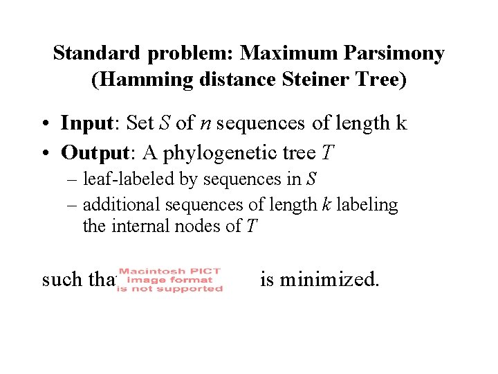
Standard problem: Maximum Parsimony (Hamming distance Steiner Tree) • Input: Set S of n sequences of length k • Output: A phylogenetic tree T – leaf-labeled by sequences in S – additional sequences of length k labeling the internal nodes of T such that is minimized.

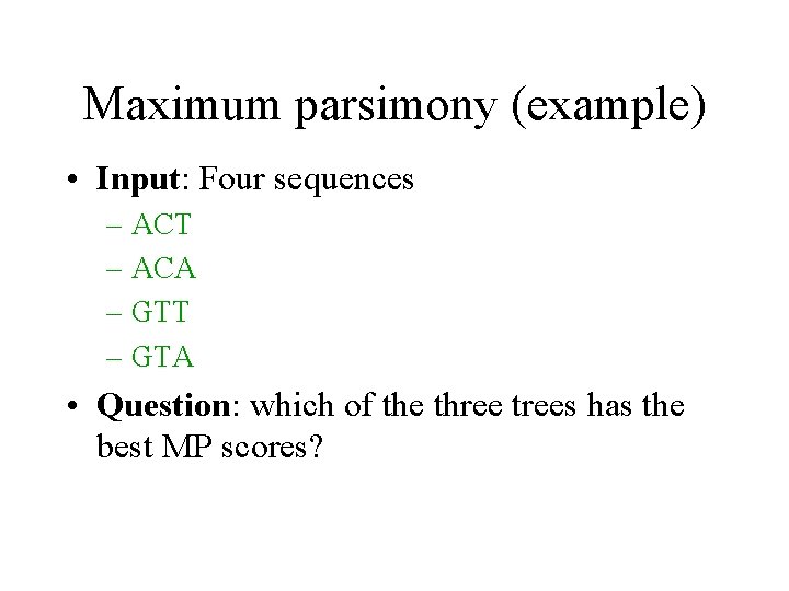
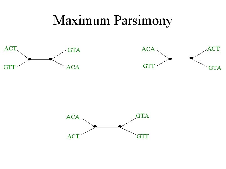
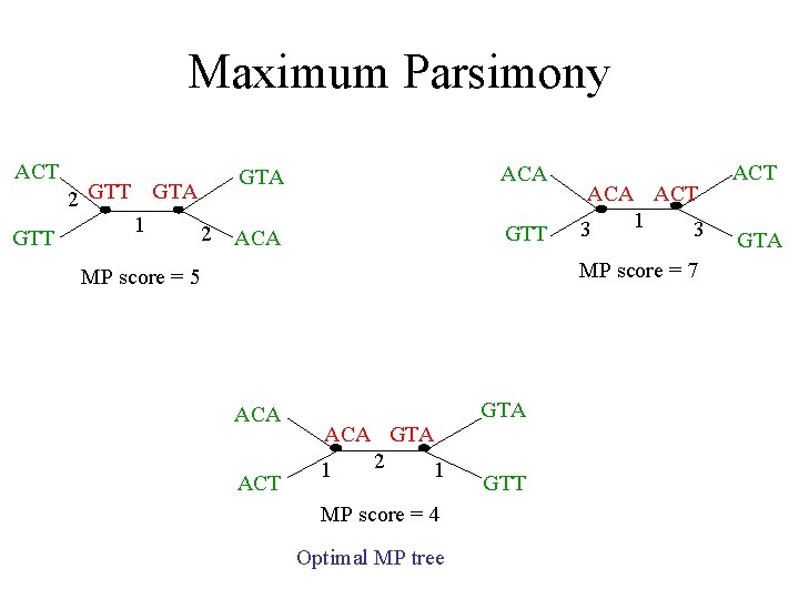
Maximum parsimony (example) • Input: Four sequences – ACT – ACA – GTT – GTA • Question: which of the three trees has the best MP scores?

Maximum Parsimony ACT GTA ACT GTT ACA GTT GTA ACA GTA ACT GTT

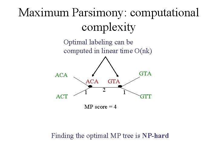
Maximum Parsimony ACT GTT 2 GTT GTA 1 2 GTA ACA GTT ACA ACT 1 3 3 MP score = 7 MP score = 5 ACA ACT GTA ACA GTA 2 1 1 MP score = 4 Optimal MP tree GTT ACT GTA

Maximum Parsimony: computational complexity Optimal labeling can be computed in linear time O(nk) ACA ACT GTA ACA 1 GTA 2 1 GTT MP score = 4 Finding the optimal MP tree is NP-hard

Local search strategies Local optimum Cost Global optimum Phylogenetic trees

Local search strategies • Hill-climbing based upon topological changes to the tree • Incorporating randomness to exit from local optima

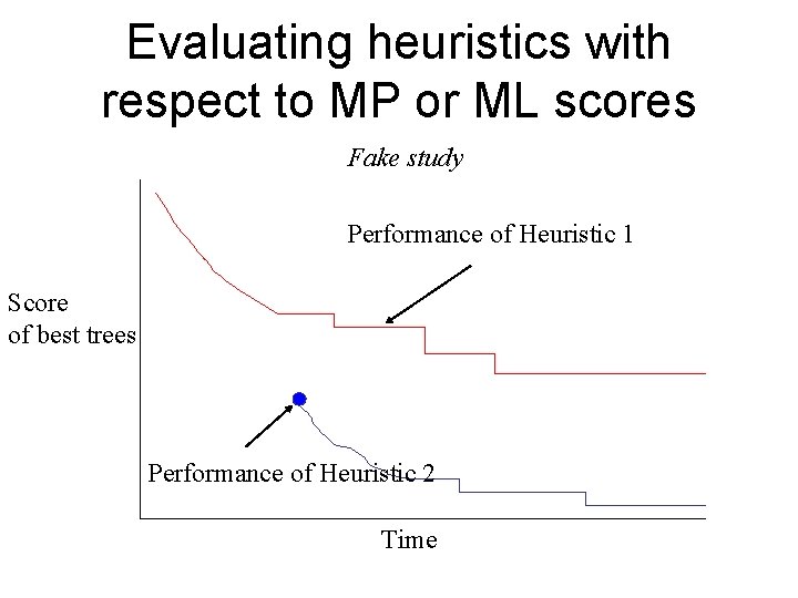
Evaluating heuristics with respect to MP or ML scores Fake study Performance of Heuristic 1 Score of best trees Performance of Heuristic 2 Time

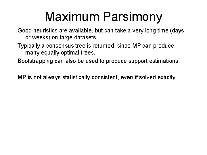
Maximum Parsimony Good heuristics are available, but can take a very long time (days or weeks) on large datasets. Typically a consensus tree is returned, since MP can produce many equally optimal trees. Bootstrapping can also be used to produce support estimations. MP is not always statistically consistent, even if solved exactly.

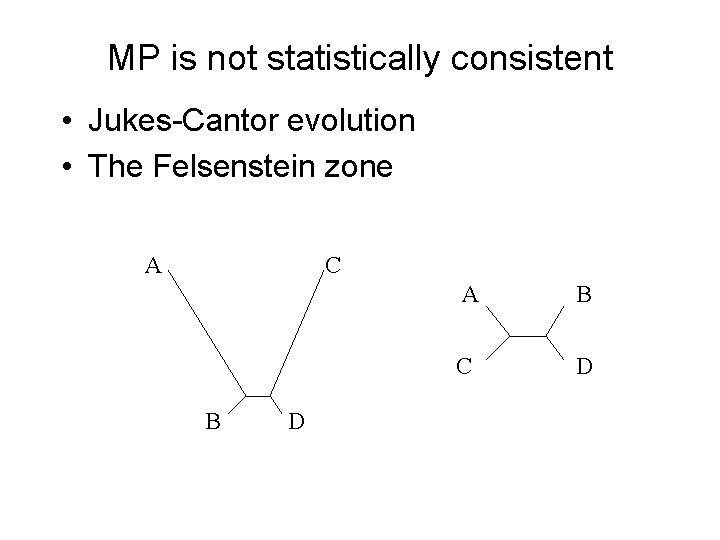
MP is not statistically consistent • Jukes-Cantor evolution • The Felsenstein zone A C B D A B C D

Maximum Likelihood ML problem: Given set S of sequences, find the model tree (T, ) such that Pr{S|T, } is maximized. Notes: • Computing Pr{S|T, } is polynomial (using Dynamic Programming) for the GTR model.

GTR Maximum Likelihood Notes (cont. ): • ML is statistically consistent under the General Time Reversible (GTR) model if solved exactly. • Finding the best GTR model tree is NP-hard (Roch). • Good heuristics exist, but can be computationally intensive (days or weeks) on large datasets. Memory requirements can be high. • Bootstrapping is used to produce support estimations on edges. Questions: What is the computational complexity of finding the best parameters on a fixed tree T? What is the sequence length requirement for ML?

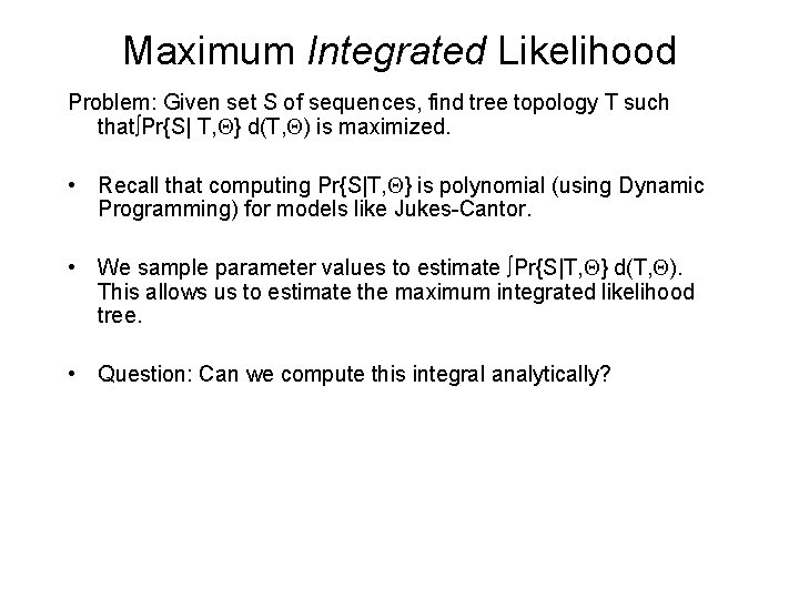
Maximum Integrated Likelihood Problem: Given set S of sequences, find tree topology T such that∫Pr{S| T, } d(T, ) is maximized. • Recall that computing Pr{S|T, } is polynomial (using Dynamic Programming) for models like Jukes-Cantor. • We sample parameter values to estimate ∫Pr{S|T, } d(T, ). This allows us to estimate the maximum integrated likelihood tree. • Question: Can we compute this integral analytically?

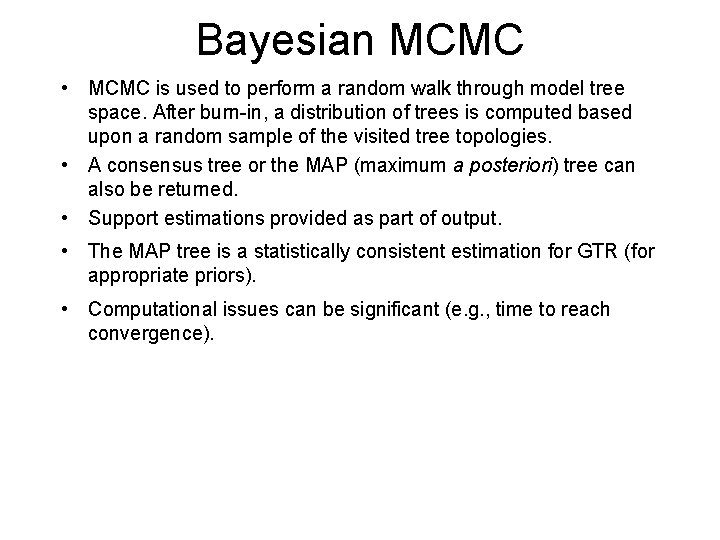
Bayesian MCMC • MCMC is used to perform a random walk through model tree space. After burn-in, a distribution of trees is computed based upon a random sample of the visited tree topologies. • A consensus tree or the MAP (maximum a posteriori) tree can also be returned. • Support estimations provided as part of output. • The MAP tree is a statistically consistent estimation for GTR (for appropriate priors). • Computational issues can be significant (e. g. , time to reach convergence).

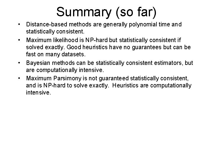
Summary (so far) • Distance-based methods are generally polynomial time and statistically consistent. • Maximum likelihood is NP-hard but statistically consistent if solved exactly. Good heuristics have no guarantees but can be fast on many datasets. • Bayesian methods can be statistically consistent estimators, but are computationally intensive. • Maximum Parsimony is not guaranteed statistically consistent, and is NP-hard to solve exactly. Heuristics are computationally intensive.

Part II • • Sequence alignment From gene trees to species trees Gene order phylogeny Reticulate evolution

X U V W X Y AGTGGAT U TATGCCCA TATGACTT AGCCCTA AGCCCGCTT Y V W

Input: unaligned sequences S 1 S 2 S 3 S 4 = = AGGCTATCACCTGACCTCCA TAGCTATCACGACCGC TAGCTGACCGC TCACGACA

Phase 1: Multiple Sequence Alignment S 1 S 2 S 3 S 4 = = AGGCTATCACCTGACCTCCA TAGCTATCACGACCGC TAGCTGACCGC TCACGACA S 1 S 2 S 3 S 4 = = -AGGCTATCACCTGACCTCCA TAG-CTATCAC--GACCGC-TAG-CT-------GACCGC----TCAC--GACCGACA

Phase 2: Construct tree S 1 S 2 S 3 S 4 = = AGGCTATCACCTGACCTCCA TAGCTATCACGACCGC TAGCTGACCGC TCACGACA S 1 S 4 S 1 S 2 S 3 S 4 S 2 S 3 = = -AGGCTATCACCTGACCTCCA TAG-CTATCAC--GACCGC-TAG-CT-------GACCGC----TCAC--GACCGACA

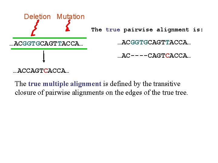
Deletion Mutation The true pairwise alignment is: …ACGGTGCAGTTACCA… …AC----CAGTCACCA… …ACCAGTCACCA… The true multiple alignment is defined by the transitive closure of pairwise alignments on the edges of the true tree.

Estimating pairwise alignments Pairwise alignment is often estimated by computing the “edit distance” (equivalently, finding a minimum cost transformation). This requires a cost for indels and substitutions.

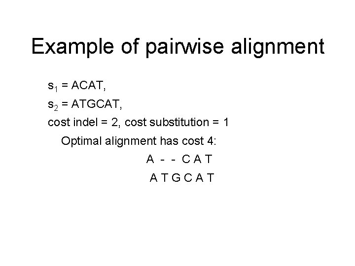
Example of pairwise alignment s 1 = ACAT, s 2 = ATGCAT, cost indel = 2, cost substitution = 1 Optimal alignment has cost 4: A - - CAT ATGCAT

Estimating alignments • Pairwise alignment is typically estimated by finding a minimum cost transformation (cost for indels and substitutions). Issues: local vs. global. • Multiple alignment: minimum cost multiple alignment is NP-hard, under various formulations.

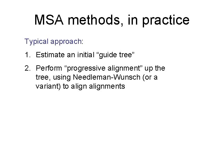
MSA methods, in practice Typical approach: 1. Estimate an initial “guide tree” 2. Perform “progressive alignment” up the tree, using Needleman-Wunsch (or a variant) to alignments

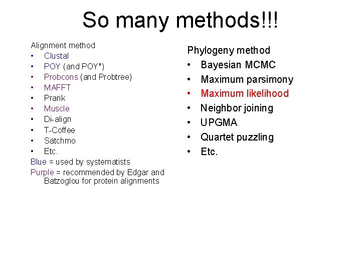
So many methods!!! Alignment method • Clustal • POY (and POY*) • Probcons (and Probtree) • MAFFT • Prank • Muscle • Di-align • T-Coffee • Satchmo • Etc. Blue = used by systematists Purple = recommended by Edgar and Batzoglou for protein alignments Phylogeny method • Bayesian MCMC • Maximum parsimony • Maximum likelihood • Neighbor joining • UPGMA • Quartet puzzling • Etc.

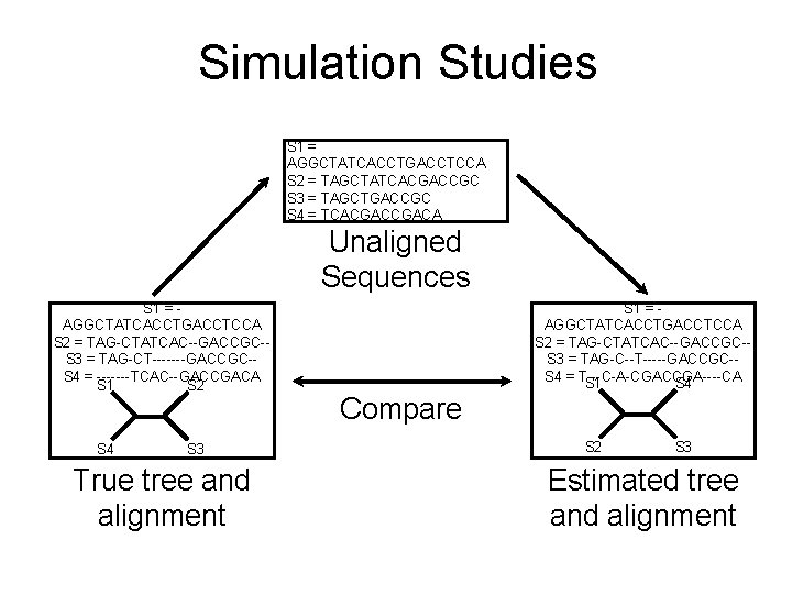
Simulation Studies S 1 = AGGCTATCACCTGACCTCCA S 2 = TAGCTATCACGACCGC S 3 = TAGCTGACCGC S 4 = TCACGACA Unaligned Sequences S 1 = AGGCTATCACCTGACCTCCA S 2 = TAG-CTATCAC--GACCGC-S 3 = TAG-CT-------GACCGC-S 4 = -------TCAC--GACCGACA S 1 S 2 S 4 S 3 True tree and alignment S 1 = AGGCTATCACCTGACCTCCA S 2 = TAG-CTATCAC--GACCGC-S 3 = TAG-C--T-----GACCGC-S 4 = T---C-A-CGACCGA----CA S 1 S 4 Compare S 2 S 3 Estimated tree and alignment

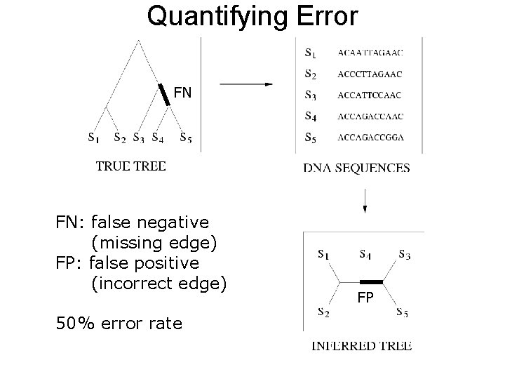
Quantifying Error FN FN: false negative (missing edge) FP: false positive (incorrect edge) 50% error rate FP

1000 taxon models, ordered by difficulty (Liu et al. , Science 2009)

Problems with the two-phase approach • Current alignment methods fail to return reasonable alignments on large datasets with high rates of indels and substitutions. • Manual alignment is time consuming and subjective. • Systematists discard potentially useful markers if they are difficult to align. This issues seriously impact large-scale phylogeny estimation (and Tree of Life projects)

Co-estimation methods • Statistical methods (e. g. , BAli. Phy, Stat. Align, Alifritz, and others) have excellent statistical performance but are extremely computationally intensive. • Steiner Tree approaches based upon edit distances (e. g. , POY) are sometimes used, but these have poor topological accuracy and are also computationally intensive. • SATé (new method) has very good empirical performance and can run on large datasets, but no guarantees under any statistical models.

SATé-1 and SATé-2 (“Next” SATé), on 1000 leaf models

Alignment-free methods • Roch and Daskalakis (RECOMB 2010) show that statistically consistent tree estimation is possible under a single-indel model • Nelesen et al. (in preparation) give practical method (DACTAL) for estimating trees without a full MSA.

DACTAL more accurate than all standard methods, and much faster than SATé Average results on 3 large RNA datasets (6 K to 28 K) CRW: Comparative RNA database, structural alignments 3 datasets with 6, 323 to 27, 643 sequences Reference trees: 75% RAx. ML bootstrap trees DACTAL (shown in red) run for 5 iterations starting from FT(Part) SATé-1 fails on the largest dataset SATé-2 runs but is not more accurate than DACTAL, and takes longer

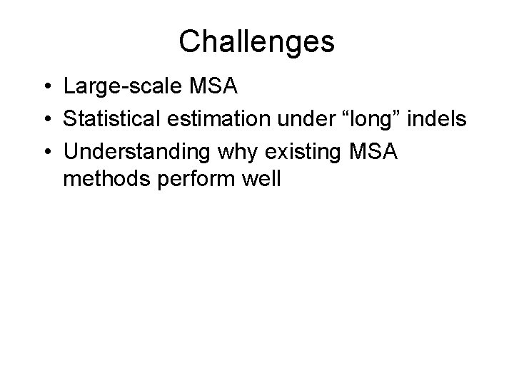
Challenges • Large-scale MSA • Statistical estimation under “long” indels • Understanding why existing MSA methods perform well

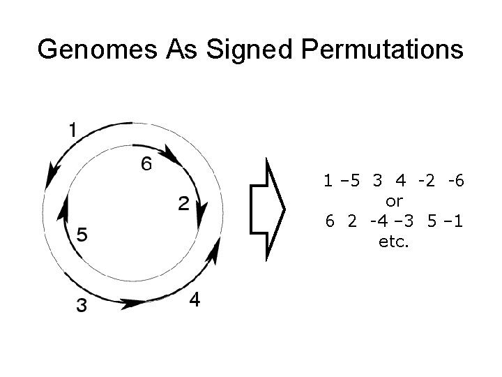
Genomes As Signed Permutations 1 – 5 3 4 -2 -6 or 6 2 -4 – 3 5 – 1 etc.

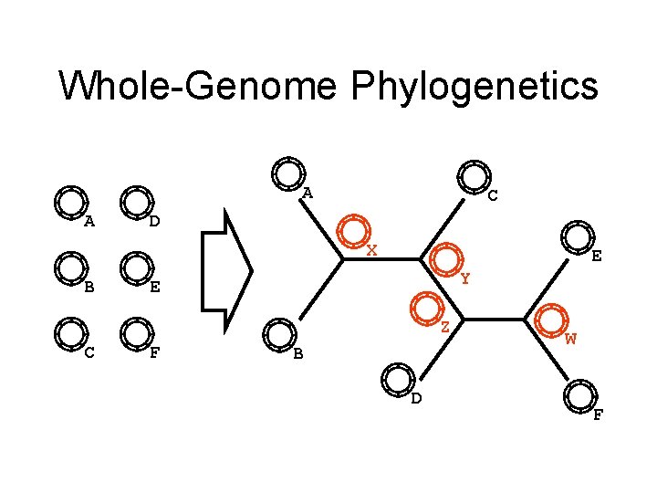
Whole-Genome Phylogenetics A A C D X B E Y E Z C F B D W F

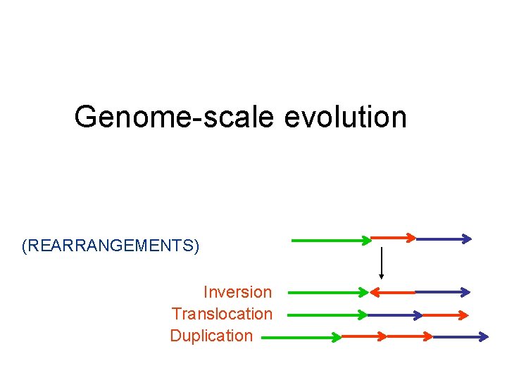
Genome-scale evolution (REARRANGEMENTS) Inversion Translocation Duplication

Other types of events • Duplications, Insertions, and Deletions (changes gene content) • Fissions and Fusions (for genomes with more than one chromosome) These events change the number of copies of each gene in each genome (“unequal gene content”)

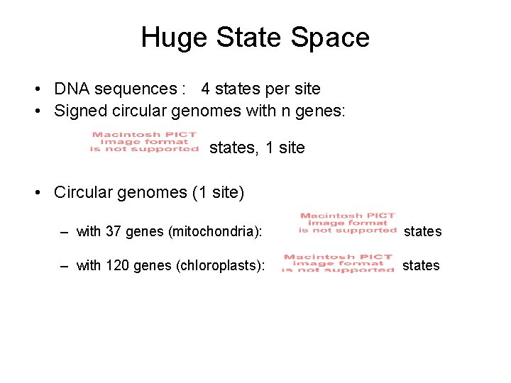
Huge State Space • DNA sequences : 4 states per site • Signed circular genomes with n genes: states, 1 site • Circular genomes (1 site) – with 37 genes (mitochondria): states – with 120 genes (chloroplasts): states

Why use gene orders? • “Rare genomic changes”: huge state space and relative infrequency of events (compared to site substitutions) could make the inference of deep evolution easier, or more accurate. • Much research shows this is true, but accurate analysis of gene order data is computationally very intensive!

Phylogeny reconstruction from gene orders • Distance-based reconstruction • Maximum Parsimony for Rearranged Genomes • Maximum Likelihood and Bayesian methods

Phylogeny reconstruction from gene orders Distance-based reconstruction: • Compute edit distances between all pairs of genomes • Correct for unseen changes (statisticallybased distance corrections) • Apply distance-based methods

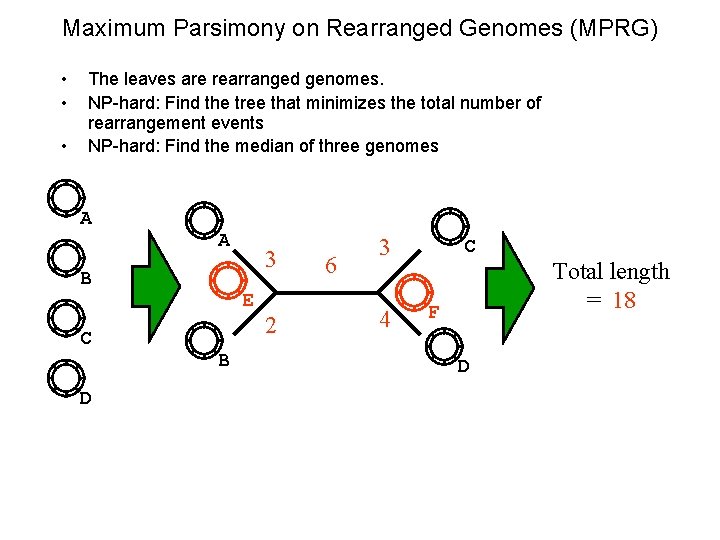
Maximum Parsimony on Rearranged Genomes (MPRG) • • • The leaves are rearranged genomes. NP-hard: Find the tree that minimizes the total number of rearrangement events NP-hard: Find the median of three genomes A A B C D 3 E B 2 6 3 4 C F D Total length = 18

Challenges • • Pairwise comparisons under complex models Estimating ancestral genomes Better models of genome evolution Combining genome-scale events with sequence-scale events • Accurate and scalable methods

Estimating species trees from multiple genes

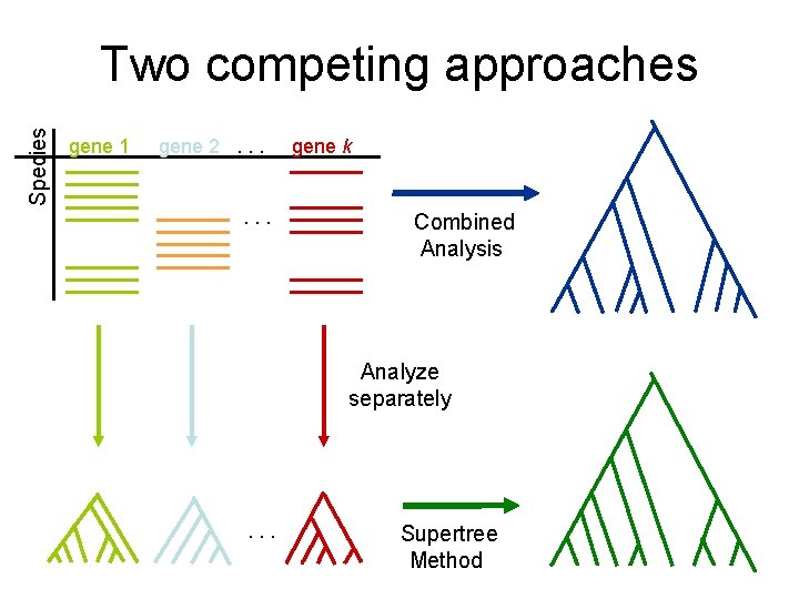
Multi-gene analyses After alignment of each gene dataset: • Combined analysis: Concatenate (“combine”) alignments for different genes, and run phylogeny estimation methods • Supertree: Compute trees on alignment and combine gene trees

Species Two competing approaches gene 1 gene 2. . . gene k Combined Analysis Analyze separately . . . Supertree Method

Supertree estimation vs. CA-ML Scaffold Density (%) (Swenson et al. , In Press, Systematic Biology)

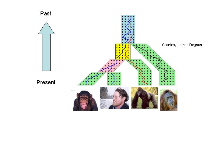
From Gene Trees to Species Trees • Gene trees can differ from species trees due to many causes, including – Duplications and losses – Incomplete lineage sorting – Horizontal gene transfer – Gene tree estimation error

Red gene tree ≠ species tree (green gene tree okay)

Past Courtesy James Degnan Present

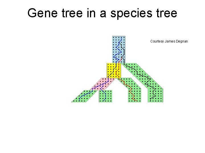
Gene tree in a species tree Courtesy James Degnan

Incomplete Lineage Sorting (deep coalescence) • Population-level process leading to gene trees differing from species trees • Factors include short times between speciation events and population size • Methods for estimating species trees under ILS include statistical approaches (*BEAST, BUCKy, STEM, GLASS, etc. ) and discrete optimization methods for MDC (minimize deep coalescence).

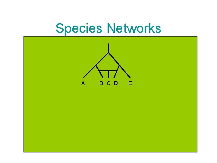
Species Networks A B C D E

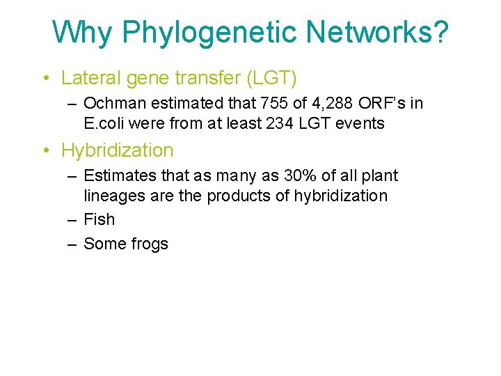
Why Phylogenetic Networks? • Lateral gene transfer (LGT) – Ochman estimated that 755 of 4, 288 ORF’s in E. coli were from at least 234 LGT events • Hybridization – Estimates that as many as 30% of all plant lineages are the products of hybridization – Fish – Some frogs

Species Networks A B C D E

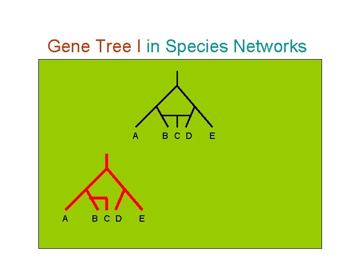
Gene Tree I in Species Networks A A B C D E E

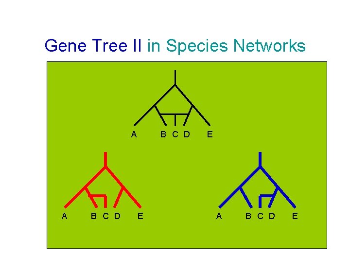
Gene Tree II in Species Networks A A B C D E E A B C D E

Species Two competing approaches gene 1 gene 2. . . gene k Combined Analysis Analyze separately . . . Supernetwork Method

Most phylogenetic network methods do not produce “explicit” models of reticulate evolution, but rather visual representations of deviations from additivity. This produces a lot of false positives!

• Current methods may be fast enough for typical (almost) whole genome analyses (small numbers of taxa and hundreds to thousands of genes). • New methods will need to be developed for larger numbers of taxa. • New methods are also needed to address the complexity of real biological data (long indels, rearrangements, duplications, heterotachy, reticulation, fragmentary data from NGS, etc. ) • Tree-of-life scale analyses will require many algorithmic advances, and present very interesting mathematical questions.

Sequence length requirements • The sequence length (number of sites) that a phylogeny reconstruction method M needs to reconstruct the true tree with probability at least 1 - depends on • M (the method) • • f = min p(e), • g = max p(e), and • n, the number of leaves

Better distance-based methods • • • Neighbor Joining Minimum Evolution Weighted Neighbor Joining Bio-NJ DCM-NJ And others

Neighbor joining has poor performance on large diameter trees [Nakhleh et al. ISMB 2001] Error Rate 0. 8 NJ 0. 6 0. 4 0. 2 0 0 400 800 No. Taxa 1200 Simulation study based upon fixed edge lengths, K 2 P model of evolution, sequence lengths fixed to 1000 nucleotides. Error rates reflect proportion of incorrect edges in inferred trees. 1600

“Boosting” MP heuristics • We use “Disk-covering methods” (DCMs) to improve heuristic searches for MP and ML Base method M DCM-M