Metaheuristic Algorithms A brief introduction on the basics

Metaheuristic Algorithms A brief introduction on the basics you need to know Panagiotis P. Repoussis School of Business Stevens Institute of Technology prepouss@stevens. edu

REFERENCES • Talbi E. -G. , 2009. Metaheuristics: from design to implementation, Vol. 74, John Wiley & Sons • Blum C. and Roli A. , 2003. Metaheuristics in combinatorial optimization: Overview and conceptual comparison, ACM Computing Surveys, 35(3): 268 -308 • Back T. , Hammel U. and Schwefel H. -P. , 2002. Evolutionary computation: comments on the history and current state, IEEE Transactions on Evolutionary Computation, 1(1): 3 -17

INTRODUCTION • Heuristics – “to find” (from ancient Greek “ευρίσκειν”) • Meta– An abstraction from another concept • beyond, in an upper level • used to complete or add to – E. g. , meta-data = “data about data” • Metaheuristics – “A heuristic around heuristics”

INTRODUCTION • Some popular frameworks – Genetic Algorithms – Simulated Annealing – Tabu Search – Scatter Search – Ant Colony Optimization – Particle Swarm Optimization – Iterated Local Search – Variable Neighborhood Search – Adaptive Memory Programming –…

INTRODUCTION • Metaheuristics… – …can address both discrete- and continuousdomain optimization problems – …are strategies that “guide” the search process – …range from simple local search procedures to complex adaptive learning processes

INTRODUCTION • Metaheuristics… – …efficiently explore the search space in order to find good (near-optimal) feasible solutions – …provide no guarantee of global or local optimality – …are agnostic to the unexplored feasible space (i. e. , no “bound” information) – …lack a metric of “goodness” of solution (often stop due to an external time or iteration limit) – …are not based on some algebraic model unlike exact methods! – …are often used in conjunction with an exact method • E. g. , use metaheuristic to provide upper bounds • E. g. , use restricted MILP as “local heuristic”

Introduction • Let’s consider the problem of find the best visiting sequence (route) to serve 14 customers. • How many possible routes exists? – (n-1)!=(15 -1)!=14!= 8, 7178 X 1010 = 88 billion solutions – If a PC can check about 1 million solution per second, then we need 8, 8*1010 routes /106 routes/ sec = 88. 000 sec or about 24, 44 hours to check them all and find the best!

COMBINATORIAL EXPLOSION 13, 509 -city TSP 19, 982. 859 mi. • What type of algorithm would you pick to solve a problem with 1049, 933 feasible solutions?

TWO BASIC DEFINITIONS •

CLASSIFICATION #5 Trajectory (S-metaheuristics) Population-based (P-metaheuristics)

TRAJECTORY METHODS

TRAJECTORY METHODS C(s 0) s 0

TRAJECTORY METHODS C(s 0) s 0 s 1 C(s 1)

TRAJECTORY METHODS C(s 0) s 0 s 1 C(s 1) s 2 C(s 2) Stop because of no improvement in region C(s 2)

TRAJECTORY METHODS C(s 0) s 0 s 1 C(s 1) s 2 C(s 2) Turns out two global optima in this problem, but none was identified • One was missed during search of region C(s 1) • One was far away from searched space

POPULATION-BASED METHODS

POPULATION-BASED METHODS 0 th population

POPULATION-BASED METHODS Get some new points

POPULATION-BASED METHODS Drop some old points

POPULATION-BASED METHODS 1 st population

POPULATION-BASED METHODS 2 nd population

POPULATION-BASED METHODS All points sampled Again, optimum may or may not have been sampled • Typically, the incumbent always remains in the population, so need only focus on last generation

CLASSIFICATION #5 Trajectory (S-metaheuristics) • Basic Local Search (3192 BC) • Simulated Annealing (1983) • Tabu Search (1986) • GRASP (1989) • Guided Local Search (1997) • Variable Neighborhood Search (1999) • Iterated Local Search (1999)

BASIC LOCAL SEARCH Iterative Improvement 12 Neighborhood 10 8 6 4 2 0 1 2 3 4 5 6 7 8 9 10 11 12 13 14 15 Improve() can be implemented as “first improvement” or “best improvement” or anything in between

BASIC LOCAL SEARCH Iterative Improvement 12 Neighborhood 10 8 6 4 2 0 1 2 3 4 5 6 7 8 9 10 11 12 13 14 15

BASIC LOCAL SEARCH Iterative Improvement 12 Neighborhood 10 8 6 4 2 0 1 2 3 4 5 6 7 8 9 10 11 12 Local optimum found, cannot improve! How to escape the local optimum “trap”? 13 14 15

ESCAPING LOCAL OPTIMA

INTENSIFY & DIVERSIFY • Merriam-Webster: Intensify • to become stronger or more extreme; to become more intense Diversify • to change (something) so that it has more different kinds of people or things

INTENSIFY & DIVERSIFY • Every metaheuristic aspires to do both • Many have parameters to control this balance • Often, these parameters can be changed dynamically during search • Initially, focus is on diversification; later, on intensification (and cycles back)

INTENSIFY & DIVERSIFY 12 10 8 6 4 2 0 1 2 3 4 5 6 7 8 9 10 11 12 13 14 15 16 17 18

INTENSIFY & DIVERSIFY

TABU SEARCH • Taboo (English): prohibited, disallowed, forbidden • Tabu (Fijian): forbidden to use due to being sacred and/or of supernatural powers • …related to similar Polynesian words tapu (Tongan), tapu (Maori), kapu (Hawaiian)

TABU SEARCH • • Used mainly for discrete problems The tabu list constitutes “short-term memory” Size of tabu list (“tenure”) is finite Since solutions in tabu list are off-limits, it helps – escape local minima by forcing uphill moves (if no improving move available) – avoid cycling (up to the period induced by tabu list size) • Solutions enter and leave the list in a FIFO order (usually)

TABU SEARCH • Small tenure localizes search (intensification) • Large tenure forces exploration of wider space (diversification) • Tenure can change dynamically during search • Size of tenure is a form of “long-term memory”

TABU SEARCH • Storing complete solutions is inefficient – implementation perspective (storage, comparisons) – algorithm perspective (largely similar solutions offer no interesting information) • Tabu search usually stores “solution attributes” – solution components or solution differences (“moves”)

TABU SEARCH Asymmetric TSP 1 A Tabu List (tenure = 3) B 0. 5 5 2 1 1 D 1. 5 C solution = {tour} move = {swap consecutive pair} attributes = {moves} Solution Trajectory A B C D A 5. 5

TABU SEARCH Asymmetric TSP 1 A Tabu List (tenure = 3) B Solution Trajectory A B C D A 5. 5 0. 5 5 2 1 1 D 1. 5 C solution = {tour} AB B A C D B 5. 0 move = {swap consecutive pair} BC A C B D A 9. 5 CD A B D C A 4. 0 DA D B C A D 4. 5 attributes = {moves}

TABU SEARCH Asymmetric TSP 1 A Tabu List (tenure = 3) B 0. 5 5 2 Solution Trajectory A B C D A 5. 5 A B D C A 4. 0 1 1 D 1. 5 C solution = {tour} AB B A C D B 5. 0 move = {swap consecutive pair} BC A C B D A 9. 5 CD A B D C A 4. 0 DA D B C A D 4. 5 attributes = {moves}

TABU SEARCH Asymmetric TSP 1 A Tabu List (tenure = 3) B CD 0. 5 5 2 1 1 D 1. 5 C solution = {tour} move = {swap consecutive pair} attributes = {moves} Solution Trajectory A B C D A 5. 5 A B D C A 4. 0

TABU SEARCH Asymmetric TSP 1 A Tabu List (tenure = 3) B CD 0. 5 5 2 Solution Trajectory A B C D A 5. 5 A B D C A 4. 0 1 1 D 1. 5 C solution = {tour} AB B A D C A 5. 0 move = {swap consecutive pair} BD A D B C A 4. 5 DC A B C D A 5. 5 CA C B D A C 9. 5 attributes = {moves}

TABU SEARCH Asymmetric TSP 1 A Tabu List (tenure = 3) B BD 0. 5 CD 5 2 1 1 D 1. 5 Solution Trajectory A B C D A 5. 5 A B D C A 4. 0 A D B C A 4. 5 C solution = {tour} AB B A D C A 5. 0 move = {swap consecutive pair} BD A D B C A 4. 5 DC A B C D A 5. 5 CA C B D A C 9. 5 attributes = {moves}

TABU SEARCH Asymmetric TSP 1 A Tabu List (tenure = 3) B BD 0. 5 CD 5 2 1 1 D 1. 5 Solution Trajectory A B C D A 5. 5 A B D C A 4. 0 A D B C A 4. 5 C solution = {tour} AD D A B C D 5. 5 move = {swap consecutive pair} DB A B D C A 4. 0 BC A D C B A 9. 5 CA C D B A C 5. 0 attributes = {moves}

TABU SEARCH Asymmetric TSP 1 A Tabu List (tenure = 3) B BD 0. 5 CD 5 2 1 1 D 1. 5 Solution Trajectory A B C D A 5. 5 A B D C A 4. 0 A D B C A 4. 5 C solution = {tour} AD D A B C D 5. 5 move = {swap consecutive pair} DB A B D C A 4. 0 BC A D C B A 9. 5 CA C D B A C 5. 0 attributes = {moves}

TABU SEARCH Asymmetric TSP 1 A Tabu List (tenure = 3) B 5 2 1 1 D 1. 5 A B C D A 5. 5 BD A B D C A 4. 0 CD A D B C A 4. 5 C D B A C 5. 0 CA 0. 5 Solution Trajectory C solution = {tour} CD D C B A D 9. 5 move = {swap consecutive pair} DB C B D A C 9. 5 BA C D A B C 5. 5 AC A D B C A 4. 5 attributes = {moves}

TABU SEARCH Asymmetric TSP 1 A Tabu List (tenure = 3) B 5 2 1 1 D 1. 5 A B C D A 5. 5 BD A B D C A 4. 0 CD A D B C A 4. 5 C D B A C 5. 0 CA 0. 5 Solution Trajectory C solution = {tour} CD D C B A D 9. 5 move = {swap consecutive pair} DB C B D A C 9. 5 BA C D A B C 5. 5 AC A D B C A 4. 5 attributes = {moves}

TABU SEARCH Asymmetric TSP 1 A Tabu List (tenure = 3) B 5 2 1 1 D 1. 5 A B C D A 5. 5 CA A B D C A 4. 0 BD A D B C A 4. 5 C D B A C 5. 0 C D A B C 5. 5 BA 0. 5 Solution Trajectory C solution = {tour} CD D C A B D 4. 0 move = {swap consecutive pair} DA C A D B C 4. 5 AB C D B A C 5. 0 BC B D A C B 9. 5 attributes = {moves}

TABU SEARCH Asymmetric TSP 2 A Tabu List (tenure = 3) B Solution Trajectory A B C D 1 2 10 4 2 D 3 3 NEW DATA! C solution = {tour} move = {swap consecutive pair} attributes = {moves} What could happen if tenure were 2 instead of 3? What could happen if tenure were 4 instead of 3? A 11

TABU SEARCH Asymmetric TSP 1 A Tabu List (tenure = 2) B 0. 5 5 2 1 1 D 1. 5 C What could happen if tenure were 2 instead of 3? Solution Trajectory A B C D A 5. 5

TABU SEARCH Asymmetric TSP 1 A Tabu List (tenure = 4) B 0. 5 5 2 1 1 D 1. 5 C What could happen if tenure were 4 instead of 3? Solution Trajectory A B C D A 5. 5

TABU SEARCH • Decreasing tenure provides for intensification, though encourages cycling • Increasing tenure provides for diversification by encouraging uphill moves • How would you design a good TS algorithm?

TABU SEARCH • Forbidding “attributes” may be overly restrictive – aspiration conditions are introduced as “wild-cards” for certain solutions, e. g. , new incumbents are always accepted, even if they possess taboo attributes

ITERATED LOCAL SEARCH • ILS is a general-purpose “multi-restart” local search framework – Provides structure in selection of next initial point • Perturbation() aspires that new initial point is – far enough to lead to a new local optimum – close enough to be better that a “random” pick

ITERATED LOCAL SEARCH • ILS is a general-purpose “multi-restart” local search framework – Provides structure in selection of next initial point • Perturbation() is non-deterministic (avoids cycling) • The “strength” of Perturbation() (i. e. , how many solution feature changes are induced) varies along search process

ITERATED LOCAL SEARCH • ILS is a general-purpose “multi-restart” local search framework – Provides structure in selection of next initial point What controls the balance between intensification and diversification?

VARIABLE NEIGHBORHOOD SEARCH • VNS is a search strategy based on dynamically changing neighborhood structures 11 10 solution quality 9 8 7 6 5 4 3 2 1 2 3 4 5 6 7 8 search coordinate 9 10 primary neighborhood (small size) 11

VARIABLE NEIGHBORHOOD SEARCH • VNS is a search strategy based on dynamically changing neighborhood structures 11 10 solution quality 9 8 7 6 5 4 3 2 1 2 3 4 5 6 7 8 search coordinate 9 10 11 primary neighborhood (small size) secondary neighborhood (large size)

VARIABLE NEIGHBORHOOD SEARCH • VNS is a search strategy based on dynamically changing neighborhood structures 11 10 solution quality 9 8 7 6 5 4 3 2 What controls the balance between intensification and diversification? 1 2 3 4 5 6 7 8 search coordinate 9 10 11 primary neighborhood (small size) secondary neighborhood (large size)

GUIDED LOCAL SEARCH • Instead of dynamically changing search directions, GLS dynamically changes (augments) objective • Main idea is to make current solution vicinity increasingly unattractive

GUIDED LOCAL SEARCH • Instead of dynamically changing search directions, GLS dynamically changes (augments) objective • Main idea is to make current solution vicinity increasingly unattractive 14 12 10 8 6 4 2 0 1 2 3 4 5 6 7 8 9 10 11 12

GUIDED LOCAL SEARCH • Instead of dynamically changing search directions, GLS dynamically changes (augments) objective • Main idea is to make current solution vicinity increasingly unattractive 14 12 10 8 6 4 2 0 1 2 3 4 5 6 7 8 9 10 11 12

GUIDED LOCAL SEARCH • Instead of dynamically changing search directions, GLS dynamically changes (augments) objective • Main idea is to make current solution vicinity increasingly unattractive 14 12 10 8 6 4 2 0 1 2 3 4 5 6 7 8 9 10 11 12

GUIDED LOCAL SEARCH • Instead of dynamically changing search directions, GLS dynamically changes (augments) objective • Main idea is to make current solution vicinity increasingly unattractive 14 12 10 8 6 4 2 0 1 2 3 4 5 6 7 8 9 10 11 12

GUIDED LOCAL SEARCH • Instead of dynamically changing search directions, GLS dynamically changes (augments) objective • Main idea is to make current solution vicinity increasingly unattractive any solution feature (e. g. , a particular solution component)

POPULATION-BASED METHODS

POPULATION-BASED METHODS 0 th population

POPULATION-BASED METHODS Get some new points

POPULATION-BASED METHODS Drop some old points

POPULATION-BASED METHODS 1 st population

POPULATION-BASED METHODS 2 nd population

POPULATION-BASED METHODS All points sampled Again, optimum may or may not have been sampled • Typically, the incumbent always remains in the population, so need only focus on last generation

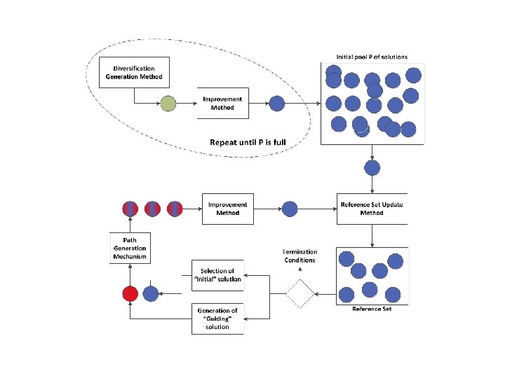
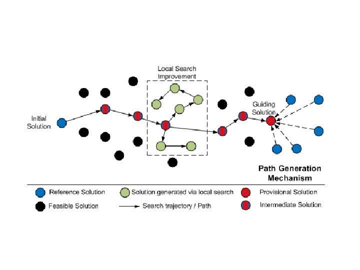
CLASSIFICATION #5 Population-based (P-metaheuristics) • Evolutionary Computation • Evolutionary Programming (1962) • Evolutionary Strategies (1973) • Genetic Algorithms (1975) • Estimation of Distribution Algorithm (1996) • Swarm Intelligence • Ant Colony Optimization (1992) • Particle Swarm Optimization (1995) • Honey-Bees Mating (2005) • Differential Evolution (1995) • Adaptive Memory Programming (1997) • Scatter Search/Path Relinking (1999)

EVOLUTIONARY COMPUTATION • Populations evolve in “generations” • New individuals (offspring) are created by combining features of current individuals (parents); – typically two parents combine to give offspring • Individuals evolve using variation operators (e. g. , “mutation”, “recombination”) acting directly on their solution representations • The next population consists of a mix of offspring and parents (“survivor selection” strategy)

EVOLUTIONARY COMPUTATION

EVOLUTIONARY COMPUTATION

EVOLUTIONARY COMPUTATION • The population size is (almost always) fixed • Selection may involve multiple copies of a given parent individual • The best individual is (almost always) carried over to the next generation • Randomness plays a significant role in generating offspring (unlike other non-EC methods) • Solutions are often represented in compact and “easily mutable” form, e. g. , bit-strings or integer permutations

EVOLUTIONARY COMPUTATION • 0 th population 12 10 8 6 4 2 0 1 2 3 4 5 6 7 8 9 10 11 12 13 14 15 16 17 18

EVOLUTIONARY COMPUTATION • Nth population 12 10 8 6 4 2 0 1 2 3 4 5 6 7 8 9 10 11 12 13 14 15 16 17 18

GENETIC ALGORITHM • Basic Evolutionary Computation Algorithm – Representation of individuals in binary code (e. g. , “ 01101” = 13, “ 11010” = 26) – Use of the “crossover” recombination operator – Mutation via “bit-flipping” – Offspring always survive EXAMPLE

Initial Population for TSP (5, 3, 4, 6, 2) (2, 4, 6, 3, 5) (4, 3, 6, 5, 2) (2, 3, 4, 6, 5) (4, 3, 6, 2, 5) (3, 4, 5, 2, 6) (3, 5, 4, 6, 2) (4, 5, 3, 6, 2) (5, 4, 2, 3, 6) (4, 6, 3, 2, 5) (3, 4, 2, 6, 5) (3, 6, 5, 1, 4)

Select Parents (5, 3, 4, 6, 2) (2, 4, 6, 3, 5) (4, 3, 6, 5, 2) (2, 3, 4, 6, 5) (4, 3, 6, 2, 5) (3, 4, 5, 2, 6) (3, 5, 4, 6, 2) (4, 5, 3, 6, 2) (5, 4, 2, 3, 6) (4, 6, 3, 2, 5) (3, 4, 2, 6, 5) (3, 6, 5, 1, 4) Try to pick the better ones.

Create Off-Spring – 1 point (5, 3, 4, 6, 2) (2, 4, 6, 3, 5) (4, 3, 6, 5, 2) (2, 3, 4, 6, 5) (4, 3, 6, 2, 5) (3, 4, 5, 2, 6) (3, 5, 4, 6, 2) (4, 5, 3, 6, 2) (5, 4, 2, 3, 6) (4, 6, 3, 2, 5) (3, 4, 2, 6, 5) (3, 6, 5, 1, 4) (3, 4, 5, 6, 2)

Create More Offspring (5, 3, 4, 6, 2) (2, 4, 6, 3, 5) (4, 3, 6, 5, 2) (2, 3, 4, 6, 5) (4, 3, 6, 2, 5) (3, 4, 5, 2, 6) (3, 5, 4, 6, 2) (4, 5, 3, 6, 2) (5, 4, 2, 3, 6) (4, 6, 3, 2, 5) (3, 4, 2, 6, 5) (3, 6, 5, 1, 4) (3, 4, 5, 6, 2) (5, 4, 2, 6, 3)

Mutate (5, 3, 4, 6, 2) (2, 4, 6, 3, 5) (4, 3, 6, 5, 2) (2, 3, 4, 6, 5) (4, 3, 6, 2, 5) (3, 4, 5, 2, 6) (3, 5, 4, 6, 2) (4, 5, 3, 6, 2) (5, 4, 2, 3, 6) (4, 6, 3, 2, 5) (3, 4, 2, 6, 5) (3, 6, 5, 1, 4) (3, 4, 5, 6, 2) (5, 4, 2, 6, 3)

Mutate (5, 3, 4, 6, 2) (2, 4, 6, 3, 5) (4, 3, 6, 5, 2) (2, 3, 4, 6, 5) (2, 3, 6, 4, 5) (3, 4, 5, 2, 6) (3, 5, 4, 6, 2) (4, 5, 3, 6, 2) (5, 4, 2, 3, 6) (4, 6, 3, 2, 5) (3, 4, 2, 6, 5) (3, 6, 5, 1, 4) (3, 4, 5, 6, 2) (5, 4, 2, 6, 3)

Eliminate (5, 3, 4, 6, 2) (2, 4, 6, 3, 5) (4, 3, 6, 5, 2) (2, 3, 4, 6, 5) (2, 3, 6, 4, 5) (3, 4, 5, 2, 6) (3, 5, 4, 6, 2) (4, 5, 3, 6, 2) (5, 4, 2, 3, 6) (4, 6, 3, 2, 5) (3, 4, 2, 6, 5) (3, 6, 5, 1, 4) (3, 4, 5, 6, 2) (5, 4, 2, 6, 3) Tend to kill off the worst ones.

Integrate (5, 3, 4, 6, 2) (2, 4, 6, 3, 5) (5, 4, 2, 6, 3) (3, 4, 5, 6, 2) (2, 3, 6, 4, 5) (3, 4, 5, 2, 6) (3, 5, 4, 6, 2) (4, 5, 3, 6, 2) (5, 4, 2, 3, 6) (4, 6, 3, 2, 5) (3, 4, 2, 6, 5) (3, 6, 5, 1, 4)

Restart (5, 3, 4, 6, 2) (2, 4, 6, 3, 5) (5, 4, 2, 6, 3) (3, 4, 5, 6, 2) (2, 3, 6, 4, 5) (3, 4, 5, 2, 6) (3, 5, 4, 6, 2) (4, 5, 3, 6, 2) (5, 4, 2, 3, 6) (4, 6, 3, 2, 5) (3, 4, 2, 6, 5) (3, 6, 5, 1, 4)

TSP Example: 30 Cities

Solution i (Distance = 941)

Solution j(Distance = 800)

Solution k(Distance = 652)

Best Solution (Distance = 420)

Overview of Performance

EVOLUTIONARY COMPUTATION • Intensification strategies: – Memetic Algorithms = use of local search procedures to improve each and every individual – Linkage Learning = use of advanced recombination operators instead of simplistic crossovers (e. g. , one-bit) to combine “good” parts of individuals • Diversification strategies: – Mutation = basic operation; usually need more than that – Crowding/Preselection = eliminate offspring that are similar to current individuals – Fitness Sharing = reduce reproductive fitness of individuals that have common features with each other, encourage preservation of “unique” features

A highly efficient and effective metaheuristic algorithm for rich VRPs • Tarantilis C. D. Anagnostopoulou A. and Repoussis P. P. (2013). Adaptive Path Relinking for Vehicle Routing and Scheduling Problems with Product Returns. Transportation Science 47, 356 -379. – Best ever reported results for the Capacitated VRP, the VRP with Time Windows and the VRP with Backhauls (comparison with more than 25 algorithms on large scale benchmark data set with up to 1000 customers)!

QUESTIONS?