Image Content Representation Representation for curves and shapes

Image Content Representation • Representation for – curves and shapes – regions – relationships between regions E. G. M. Petrakis Image Representation & Recognition 1

Reliable Representation • Uniqueness: must uniquely specify an image – otherwise dissimilar images might have similar representations • Invariance: must be invariant to viewing conditions: translation, rotation, scale invariant, viewing angle changes and symmetric transformations • Efficiency: computationally efficient E. G. M. Petrakis Image Representation & Recognition 2

More Criteria • Robustness: resistance to moderate amounts of deformation and noise – distortions and noise should at least result in variations in the representations of similar magnitude • Scalability: must contain information about the image at many levels of detail – images are deemed similar even if they appear at different view-scales (resolution) E. G. M. Petrakis Image Representation & Recognition 3

Image Recognition • Match the representation of an unknown image with representations computed from known images (model based recognition) • Matching takes in two representations and computes their distance – the more similar the images are the lower their distance is (and the reverse) E. G. M. Petrakis Image Representation & Recognition 4

Shape Representation • The shapes are represented by contours or curves • Contour: a linked list of edge pixels – open or closed region boundaries – much space overhead • Curve: the mathematical model of a contour – polygons – splines E. G. M. Petrakis Image Representation & Recognition 5

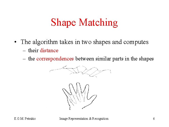
Shape Matching • The algorithm takes in two shapes and computes – their distance – the correspondences between similar parts in the shapes E. G. M. Petrakis Image Representation & Recognition 6

Polylines • Sequence of line segments approximating a contour joined end to end • Polyline: P={(x 1, y 1), (x 2, y 2), …. , (xn, yn)} – for closed contours x 1=xn, xn=yn • Vertices: points where line segments are joined E. G. M. Petrakis Image Representation & Recognition 7

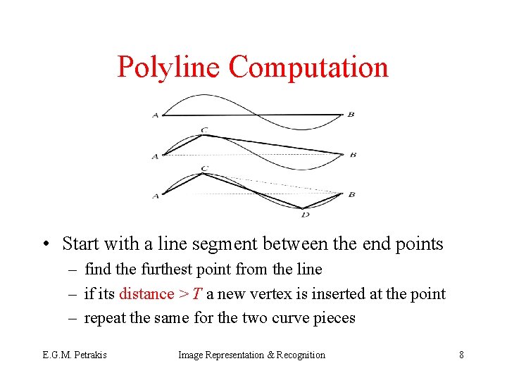
Polyline Computation • Start with a line segment between the end points – find the furthest point from the line – if its distance > T a new vertex is inserted at the point – repeat the same for the two curve pieces E. G. M. Petrakis Image Representation & Recognition 8

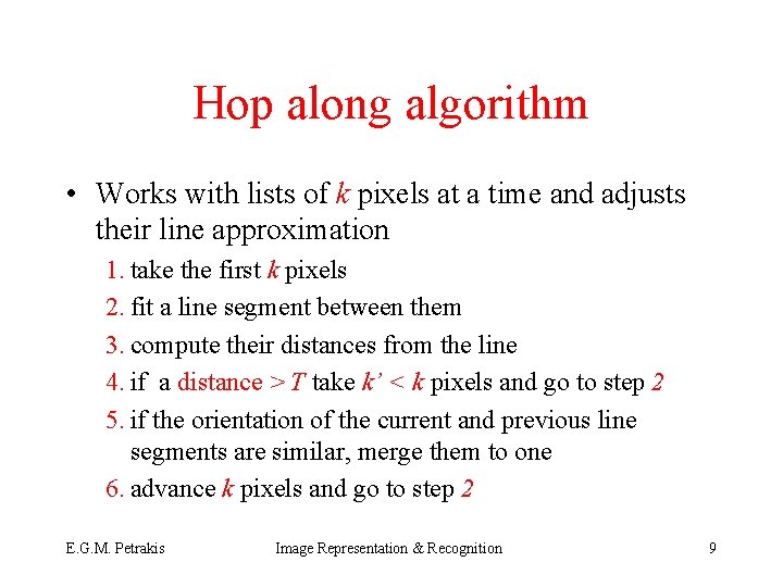
Hop along algorithm • Works with lists of k pixels at a time and adjusts their line approximation 1. take the first k pixels 2. fit a line segment between them 3. compute their distances from the line 4. if a distance > T take k’ < k pixels and go to step 2 5. if the orientation of the current and previous line segments are similar, merge them to one 6. advance k pixels and go to step 2 E. G. M. Petrakis Image Representation & Recognition 9

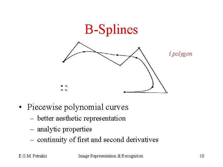
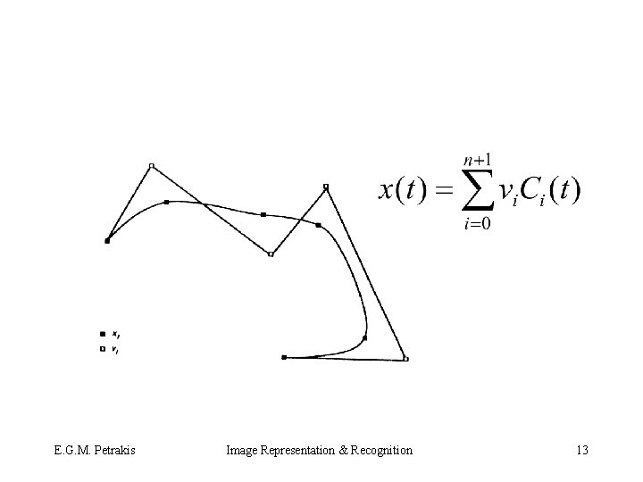
B-Splines guided polygon spline • Piecewise polynomial curves – better aesthetic representation – analytic properties – continuity of first and second derivatives E. G. M. Petrakis Image Representation & Recognition 10

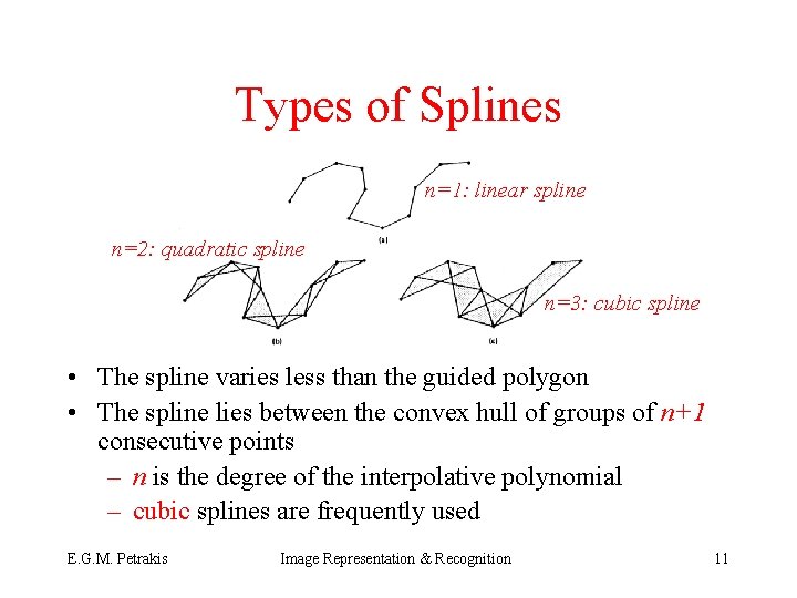
Types of Splines n=1: linear spline n=2: quadratic spline n=3: cubic spline • The spline varies less than the guided polygon • The spline lies between the convex hull of groups of n+1 consecutive points – n is the degree of the interpolative polynomial – cubic splines are frequently used E. G. M. Petrakis Image Representation & Recognition 11

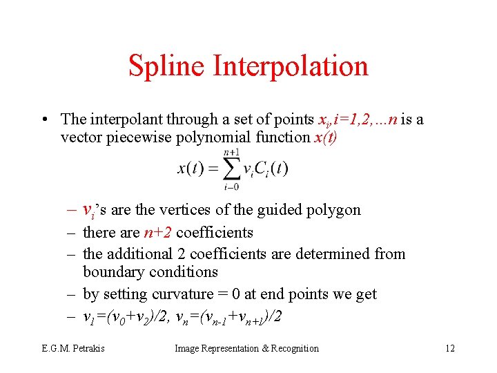
Spline Interpolation • The interpolant through a set of points xi, i=1, 2, …n is a vector piecewise polynomial function x(t) – vi’s are the vertices of the guided polygon – there are n+2 coefficients – the additional 2 coefficients are determined from boundary conditions – by setting curvature = 0 at end points we get – v 1=(v 0+v 2)/2, vn=(vn-1+vn+1)/2 E. G. M. Petrakis Image Representation & Recognition 12

E. G. M. Petrakis Image Representation & Recognition 13

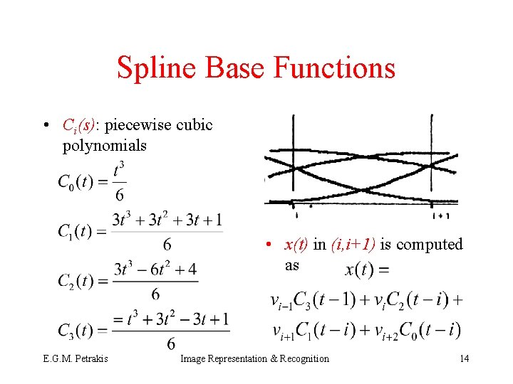
Spline Base Functions • Ci(s): piecewise cubic polynomials • x(t) in (i, i+1) is computed as E. G. M. Petrakis Image Representation & Recognition 14

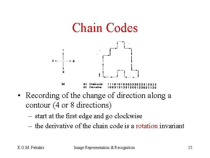
Chain Codes • Recording of the change of direction along a contour (4 or 8 directions) – start at the first edge and go clockwise – the derivative of the chain code is a rotation invariant E. G. M. Petrakis Image Representation & Recognition 15

Comments • Independency of starting point is achieved by “rotating” the code until the sequence of codes forms the minimum possible integer • Sensitive to noise and scale • Extension: approximate the boundary using chain codes (li, ai), (Tsai & Yu, IEE PAMI 7(4): 453 -462, 1985) – li: length – ai: angle difference between consecutive vectors E. G. M. Petrakis Image Representation & Recognition 16

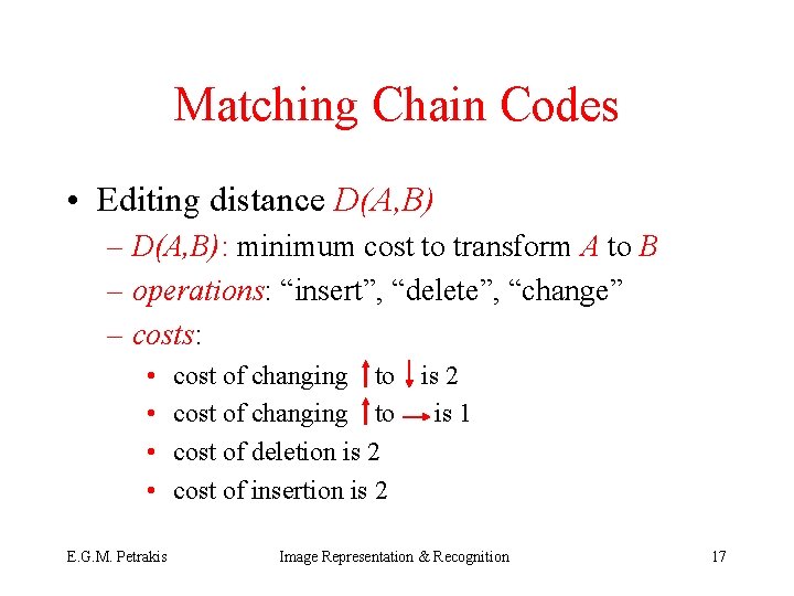
Matching Chain Codes • Editing distance D(A, B) – D(A, B): minimum cost to transform A to B – operations: “insert”, “delete”, “change” – costs: • • E. G. M. Petrakis cost of changing to cost of deletion is 2 cost of insertion is 2 is 1 Image Representation & Recognition 17

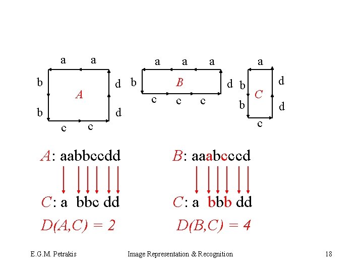
a b a a d b A c b d c a B c a a d b c b C d c c A: aabbccdd B: aaabcccd C: a bbc dd D(A, C) = 2 C: a bbb dd D(B, C) = 4 E. G. M. Petrakis d Image Representation & Recognition 18

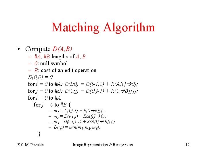
Matching Algorithm • Compute D(A, B) – #A, #B lengths of A, B – 0: null symbol – R: cost of an edit operation D(0, 0) = 0 for i = 0 to #A: D(i: 0) = D(i-1, 0) + R(A[i] 0); for j = 0 to #B: D(0: j) = D(0, j-1) + R(0 B[j]); for i = 0 to #A for j = 0 to #B { – – } E. G. M. Petrakis m 1 = D(i, j-1) + R(0 B[j]); m 2 = D(i-1, j) + R(A[i] 0); m 3 = D(i-1, j-1) + R(A[i] B[j]); D(i, j) = min{m 1, m 2, m 3}; Image Representation & Recognition 19

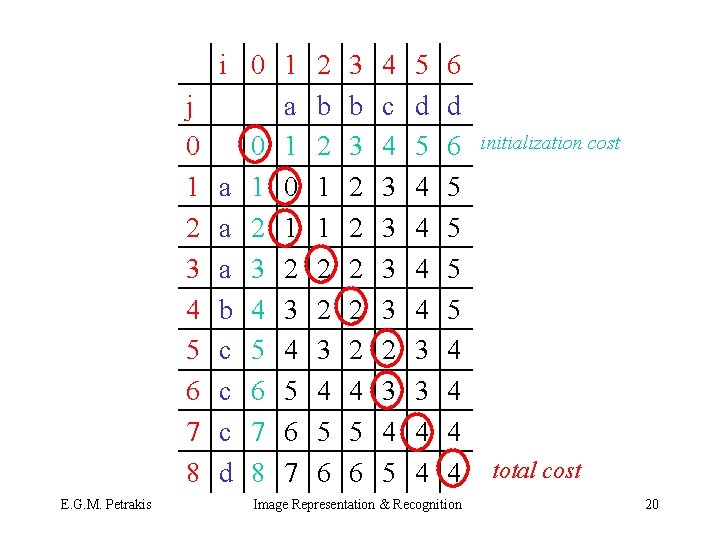
j 0 1 2 3 4 5 6 7 8 E. G. M. Petrakis i 0 1 a 1 0 a 2 1 a 3 2 b 4 3 c 5 4 c 6 5 c 7 6 d 8 7 2 b 2 1 1 2 2 3 4 5 6 3 b 3 2 2 2 4 5 6 4 c 4 3 3 2 3 4 5 5 d 5 4 4 3 3 4 4 6 d 6 5 5 4 4 Image Representation & Recognition initialization cost total cost 20

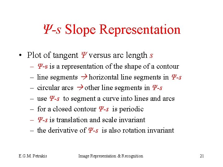
Ψ-s Slope Representation • Plot of tangent Ψ versus arc length s – – – – Ψ-s is a representation of the shape of a contour line segments horizontal line segments in Ψ-s circular arcs other line segments in Ψ-s use Ψ-s to segment a curve into lines and arcs for a closed contour Ψ-s is periodic Ψ-s is translation and scale invariant the derivative of Ψ-s is also rotation invariant E. G. M. Petrakis Image Representation & Recognition 21

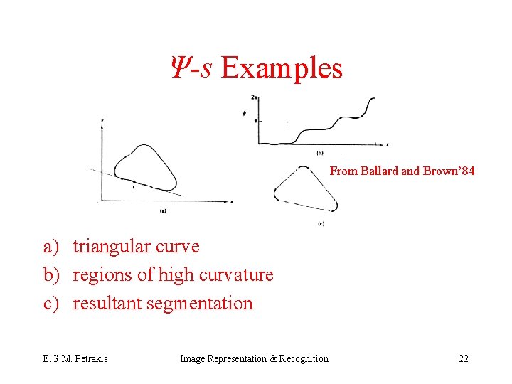
Ψ-s Examples From Ballard and Brown’ 84 a) triangular curve b) regions of high curvature c) resultant segmentation E. G. M. Petrakis Image Representation & Recognition 22

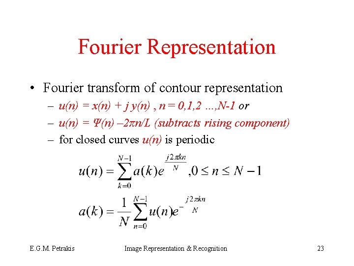
Fourier Representation • Fourier transform of contour representation – u(n) = x(n) + j y(n) , n = 0, 1, 2 …, N-1 or – u(n) = Ψ(n) – 2πn/L (subtracts rising component) – for closed curves u(n) is periodic E. G. M. Petrakis Image Representation & Recognition 23

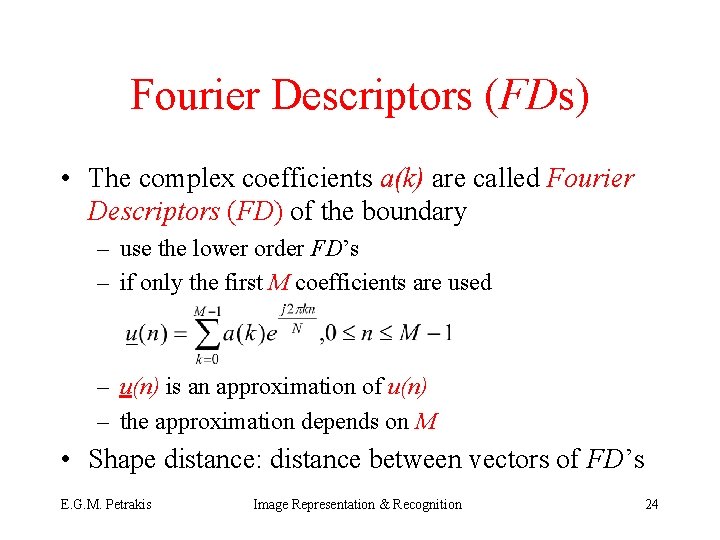
Fourier Descriptors (FDs) • The complex coefficients a(k) are called Fourier Descriptors (FD) of the boundary – use the lower order FD’s – if only the first M coefficients are used – u(n) is an approximation of u(n) – the approximation depends on M • Shape distance: distance between vectors of FD’s E. G. M. Petrakis Image Representation & Recognition 24

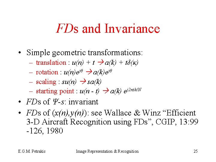
FDs and Invariance • Simple geometric transformations: – – translation : u(n) + t a(k) + tδ(κ) rotation : u(n)ejθ a(k)ejθ scaling : su(n) sa(k) starting point : u(n - t) a(k) ej 2πtk/N • FDs of Ψ-s: invariant • FDs of (x(n), y(n)): see Wallace & Winz “Efficient 3 -D Aircraft Recognition using FDs”, CGIP, 13: 99 -126, 1980 E. G. M. Petrakis Image Representation & Recognition 25

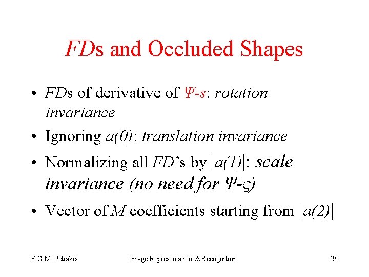
FDs and Occluded Shapes • FDs of derivative of Ψ-s: rotation invariance • Ignoring a(0): translation invariance • Normalizing all FD’s by |a(1)|: scale invariance (no need for Ψ-ς) • Vector of M coefficients starting from |a(2)| E. G. M. Petrakis Image Representation & Recognition 26

Moment Invariants [Hu 62] • An object is represented by its binary image R • A set of 7 features can be defined based on central moments E. G. M. Petrakis Image Representation & Recognition 27

Central Moments [Hu 62] • Invariant to translation and rotation • Use ηpq=μpq/μγ 00 where γ=(p+q)/2 + 1 for p+q=2, 3… instead of μ’s in the above formulas to achieve scale invariance E. G. M. Petrakis Image Representation & Recognition 28

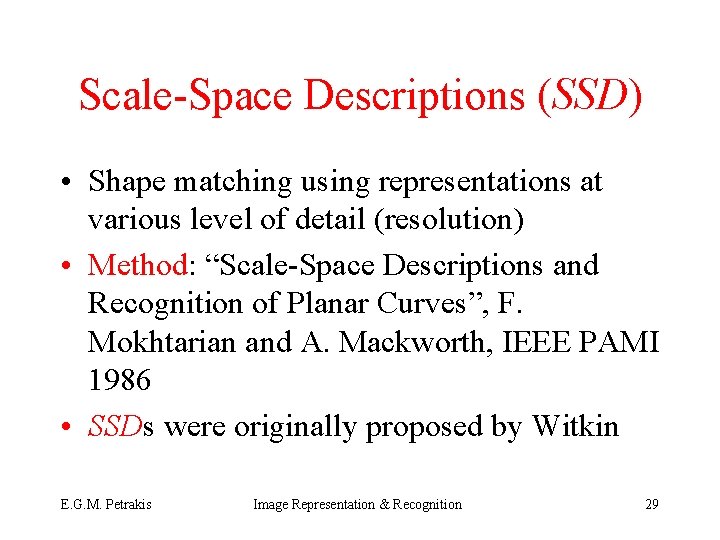
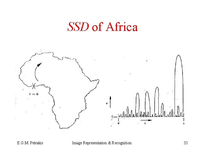
Scale-Space Descriptions (SSD) • Shape matching using representations at various level of detail (resolution) • Method: “Scale-Space Descriptions and Recognition of Planar Curves”, F. Mokhtarian and A. Mackworth, IEEE PAMI 1986 • SSDs were originally proposed by Witkin E. G. M. Petrakis Image Representation & Recognition 29

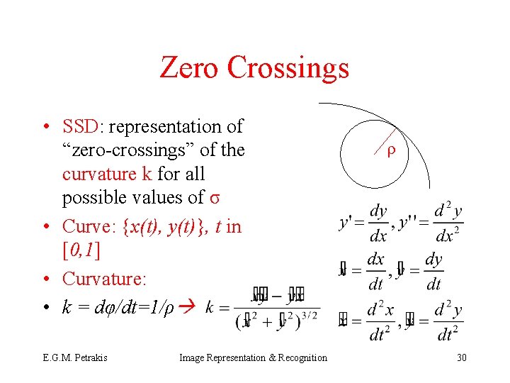
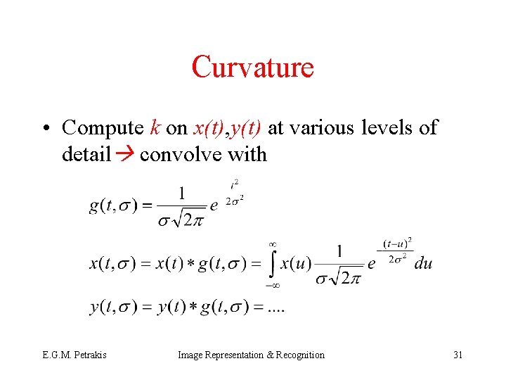
Zero Crossings • SSD: representation of “zero-crossings” of the curvature k for all possible values of σ • Curve: {x(t), y(t)}, t in [0, 1] • Curvature: • k = dφ/dt=1/ρ E. G. M. Petrakis Image Representation & Recognition ρ 30

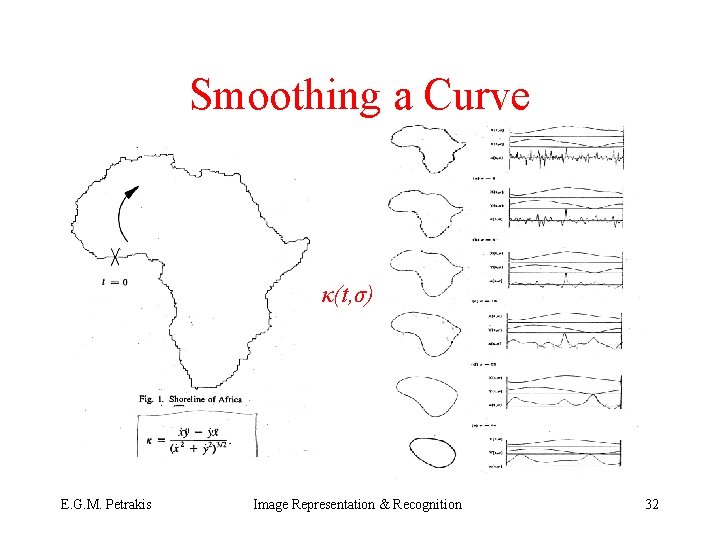
Curvature • Compute k on x(t), y(t) at various levels of detail convolve with E. G. M. Petrakis Image Representation & Recognition 31

Smoothing a Curve κ(t, σ) E. G. M. Petrakis Image Representation & Recognition 32

SSD of Africa E. G. M. Petrakis Image Representation & Recognition 33

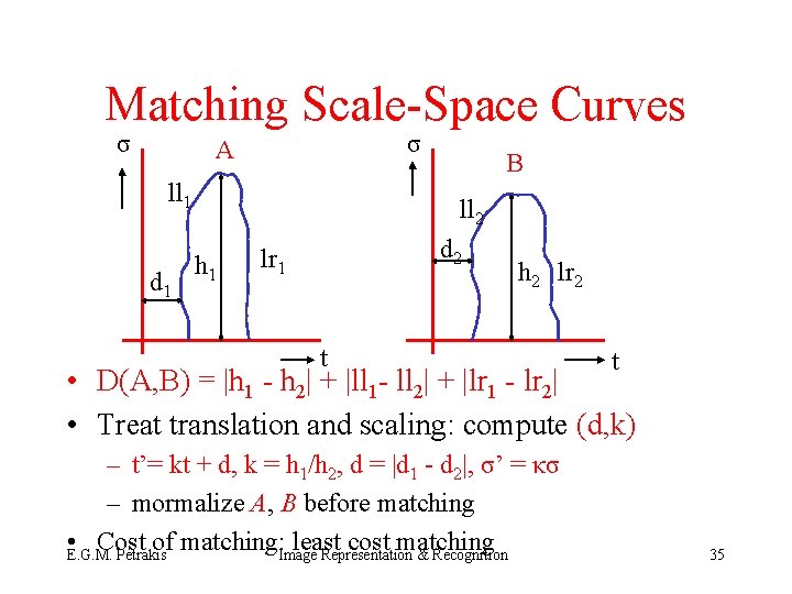
Matching SSDs • Variant of A* algorithm 1. compare the two higher curves first 2. compare the curves included starting from the two higher curves etc. until all included curves are matched 3. compare the curves next to the two higher • Some curves may be missing – assign a cost for missing curves E. G. M. Petrakis Image Representation & Recognition 34

Matching Scale-Space Curves σ σ A ll 1 d 1 B ll 2 h 1 d 2 lr 1 h 2 lr 2 t t • D(A, B) = |h 1 - h 2| + |ll 1 - ll 2| + |lr 1 - lr 2| • Treat translation and scaling: compute (d, k) – t’= kt + d, k = h 1/h 2, d = |d 1 - d 2|, σ’ = κσ – mormalize A, B before matching • Cost of matching: Image least cost matching E. G. M. Petrakis Representation & Recognition 35

Relational Structures • Representations of the relationships between objects – Attributed Relational Graphs (ARGs) – Semantic Nets (SNs) – Propositional Logic • May include or combined with representations of objects E. G. M. Petrakis Image Representation & Recognition 36

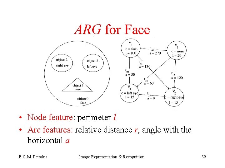
Attributed Relational Graphs (ARGs) • Objects correspond to nodes, relationships between objects correspond to arcs between nodes – both nodes and arcs may be labeled – label types depend on application and designer – usually feature vectors – recognition is based on graph matching which is NP-hard E. G. M. Petrakis Image Representation & Recognition 37

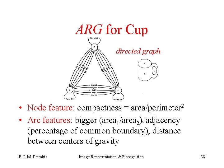
ARG for Cup directed graph • Node feature: compactness = area/perimeter 2 • Arc features: bigger (area 1/area 2)’ adjacency (percentage of common boundary), distance between centers of gravity E. G. M. Petrakis Image Representation & Recognition 38

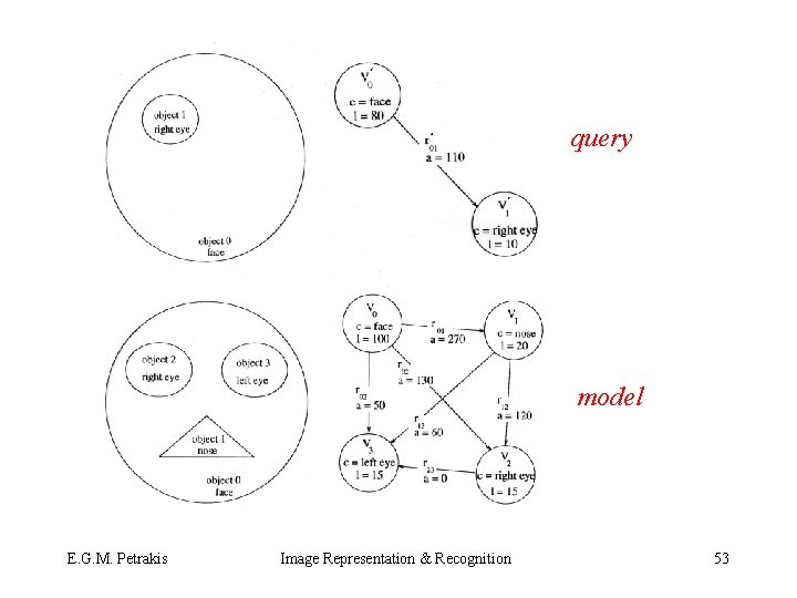
ARG for Face • Node feature: perimeter l • Arc features: relative distance r, angle with the horizontal a E. G. M. Petrakis Image Representation & Recognition 39

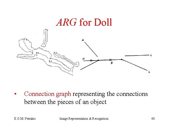
ARG for Doll • Connection graph representing the connections between the pieces of an object E. G. M. Petrakis Image Representation & Recognition 40

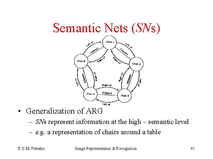
Semantic Nets (SNs) • Generalization of ARG – SNs represent information at the high – semantic level – e. g. a representation of chairs around a table E. G. M. Petrakis Image Representation & Recognition 41

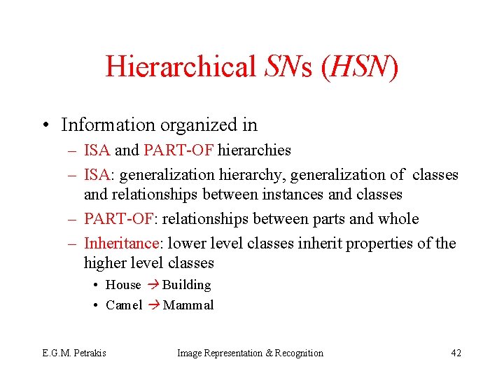
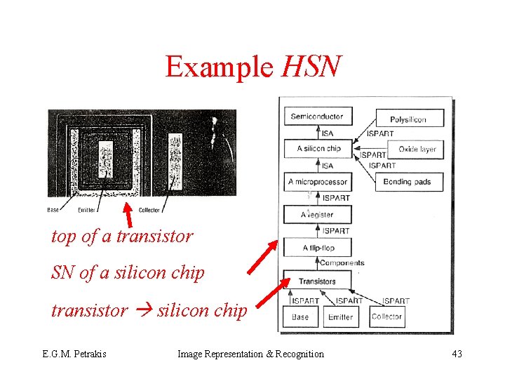
Hierarchical SNs (HSN) • Information organized in – ISA and PART-OF hierarchies – ISA: generalization hierarchy, generalization of classes and relationships between instances and classes – PART-OF: relationships between parts and whole – Inheritance: lower level classes inherit properties of the higher level classes • House Building • Camel Mammal E. G. M. Petrakis Image Representation & Recognition 42

Example HSN top of a transistor SN of a silicon chip transistor silicon chip E. G. M. Petrakis Image Representation & Recognition 43

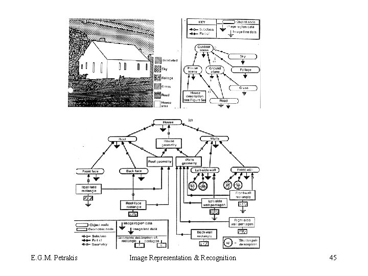
Long / Short Term Memory • Long Term Memory (LTM): schema or model representation of an image at high semantic level – virtual classes in C++ • Short Term Memory (STM): representation of instances to LTM objects – instances to virtual classes E. G. M. Petrakis Image Representation & Recognition 44

E. G. M. Petrakis Image Representation & Recognition 45

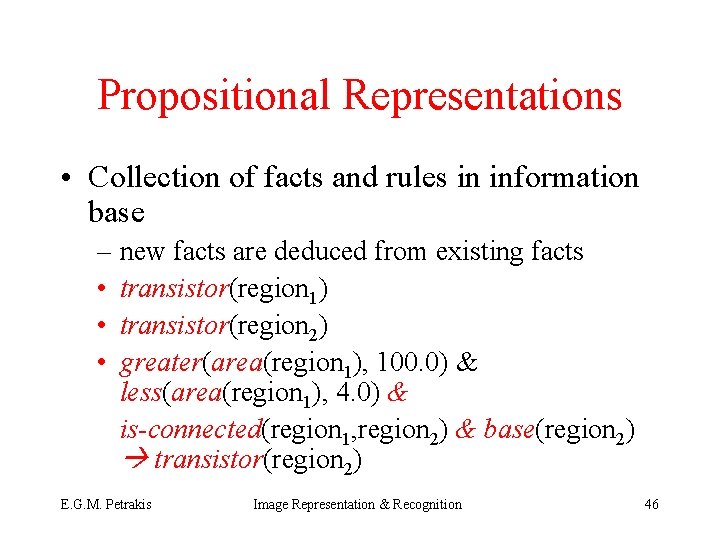
Propositional Representations • Collection of facts and rules in information base – new facts are deduced from existing facts • transistor(region 1) • transistor(region 2) • greater(area(region 1), 100. 0) & less(area(region 1), 4. 0) & is-connected(region 1, region 2) & base(region 2) transistor(region 2) E. G. M. Petrakis Image Representation & Recognition 46

Comments • Pros: – clear and compact – expandable representations of image knowledge • Cons: – non-hierarchical – not easy to treat uncertainty and incompatibilities – complexity of matching E. G. M. Petrakis Image Representation & Recognition 47

Matching Relational Structures • Matching between A, B is transformed to a graph or sub-graph isomorphism problem – graph isomorphism: one to one mapping of nodes and arcs between the structures of A, B (NP-hard!) – sub-graph isomorphism: isomorphism of a subgraph of A and B (harder!!) – double sub-graph isomorphism: isomorphism of a sub-graph of A and a sub-graph of B (even harder!!!) E. G. M. Petrakis Image Representation & Recognition 48

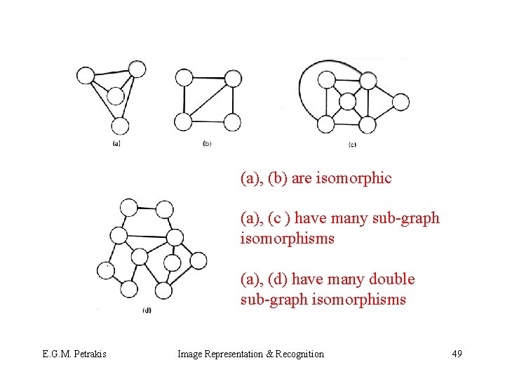
(a), (b) are isomorphic (a), (c ) have many sub-graph isomorphisms (a), (d) have many double sub-graph isomorphisms E. G. M. Petrakis Image Representation & Recognition 49

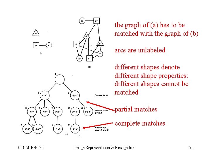
Matching Algorithm • Find all sub-graph isomorphisms • Branch and bound search with backtracking – at each step expand a partial solution at all possible directions – when search fails (a partial solution can’t be expanded) backtrack to an earlier partial solution – the cost of complete solution is an upper bound to prune the expansion of non-promising solutions with greater cost – keep the least complete solution E. G. M. Petrakis Image Representation & Recognition 50

the graph of (a) has to be matched with the graph of (b) arcs are unlabeled different shapes denote different shape properties: different shapes cannot be matched partial matches complete matches E. G. M. Petrakis Image Representation & Recognition 51

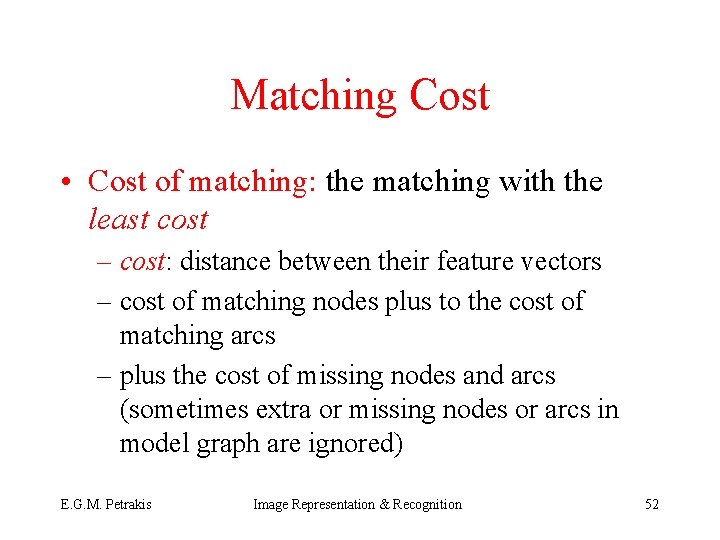
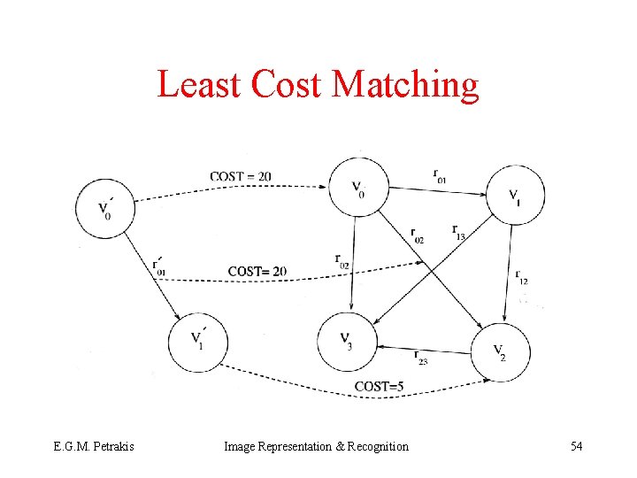
Matching Cost • Cost of matching: the matching with the least cost – cost: distance between their feature vectors – cost of matching nodes plus to the cost of matching arcs – plus the cost of missing nodes and arcs (sometimes extra or missing nodes or arcs in model graph are ignored) E. G. M. Petrakis Image Representation & Recognition 52

query model E. G. M. Petrakis Image Representation & Recognition 53

Least Cost Matching E. G. M. Petrakis Image Representation & Recognition 54