IT 472 Digital Image Processing Chapter 11 Representation

IT 472: Digital Image Processing Chapter 11: Representation & Description

Why? • A typical image processing pipeline: Pre-processing: Image Enhancement Segmentation: Detect object of interest Recognition & Interpretation

Why? • A typical image processing pipeline: Pre-processing: Image Enhancement Segmentation: Detect object of interest Recognition & Interpretation • We need to represent the segmented region in an appropriate form so that tasks like recognition etc. are possible.

Why • If we need “shape” information, then some representation of boundary of the segmented region is enough. • If we also need colour and texture information within the segmented region, then we need to represent the entire region.

Description • Description is simply an efficient representation and can also be thought of as features. • Example: Boundary – length, convex/concave, curvature extrema, etc. • Basic guideline: Descriptors should be invariant to transformations to which you want your algorithm (recognition etc. ) to be invariant.

Boundary following (Moore alg. ) • Input: Binary image with 0(black) for objects and 1 (white) for background. • Output: Sequence (C 1, C 2, …, Cn) of boundary pixels The images used to demonstrate Moore’s algorithm have been taken from the presentation by Jason Pereira, UT Arlington

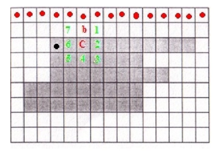
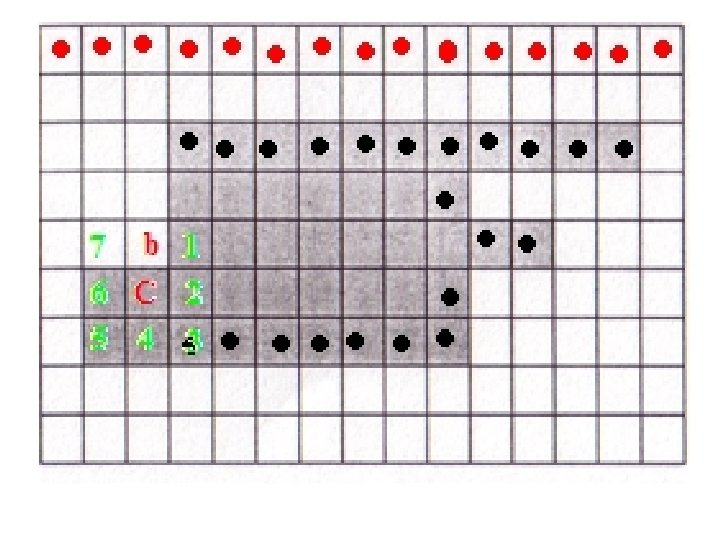
Moore’s algorithm • Start scanning from top to bottom, left to right

• Continue till you come to the first object pixel

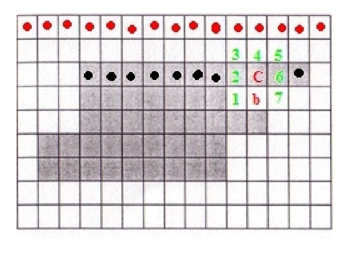
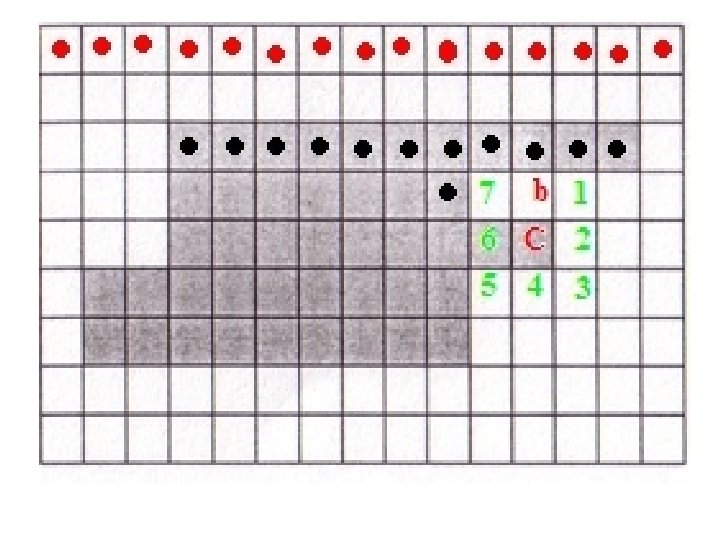
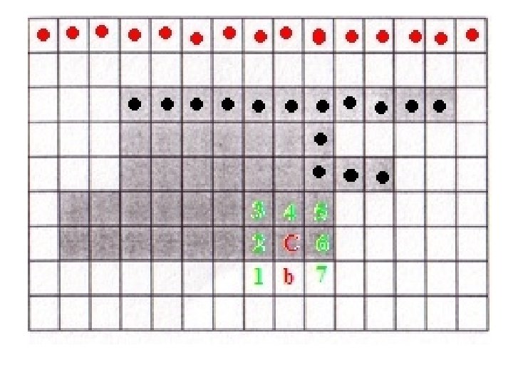
• Let the first object pixel be denoted by X, and let current pixel being scanned be denoted by C. • Because of the scanning method adopted, the pixel to the left of X will always be 1, let that pixel be denoted by b 0 (b in the illustration). • The 8 neighbors of C are put in clockwise order n 1, n 2, …, n 8 starting from the pixel clockwise-next to b.

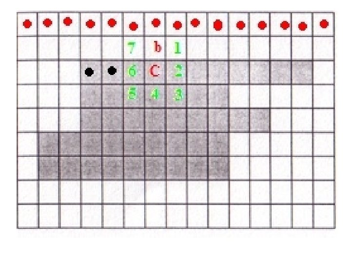
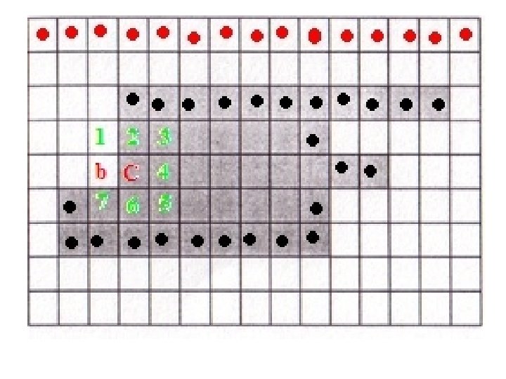
• Check the 8 neighbors in this order and find the first ni that is an object pixel. • In this case, i = 4.

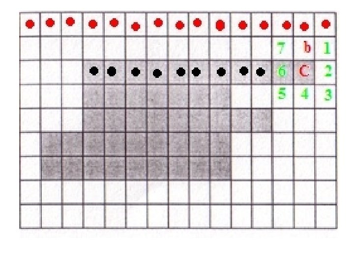
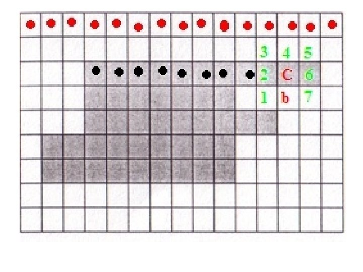
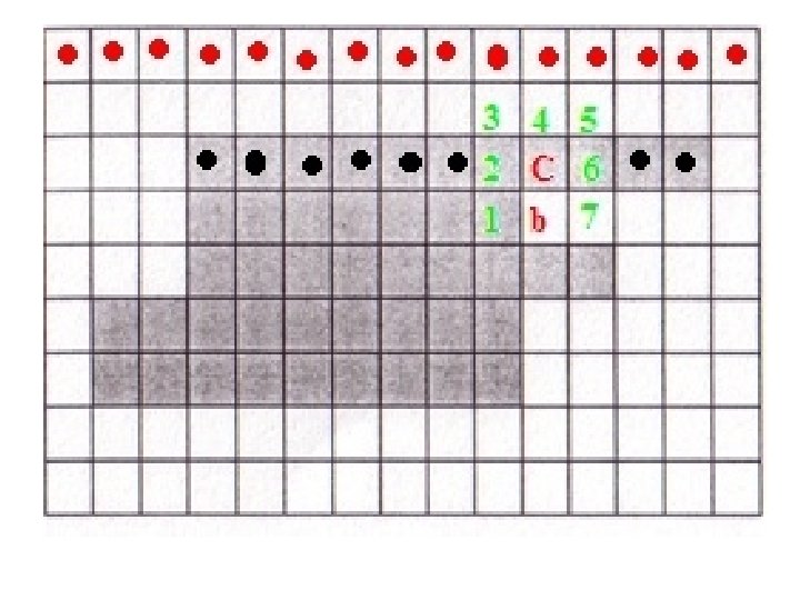
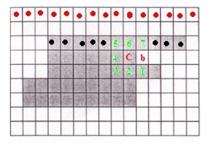
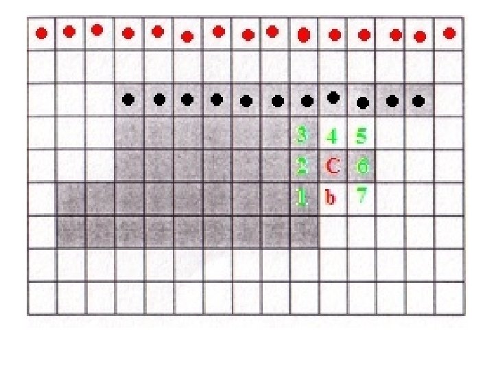
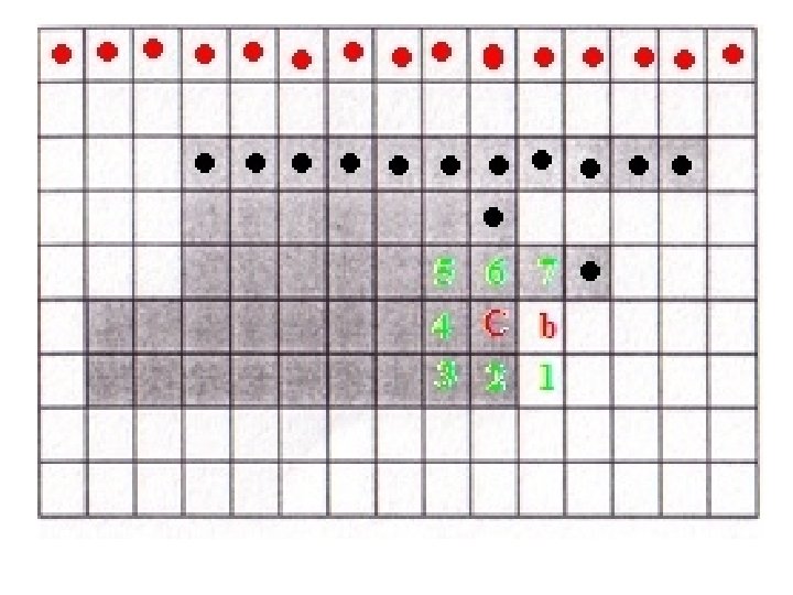
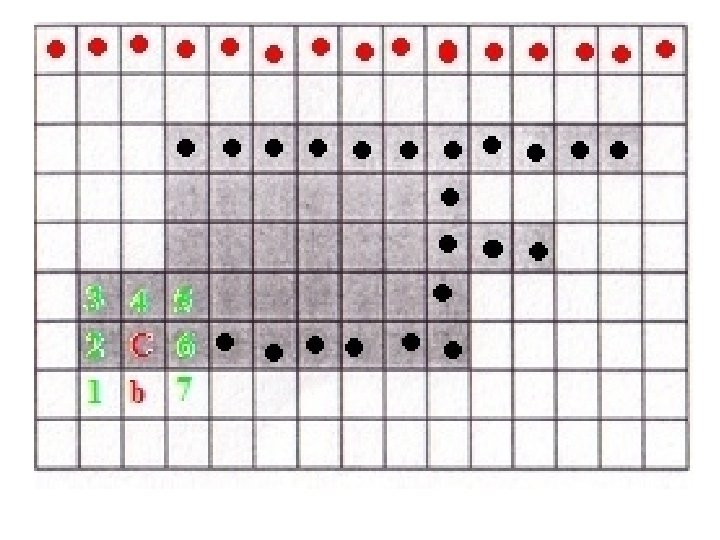
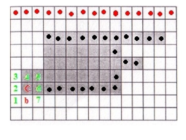
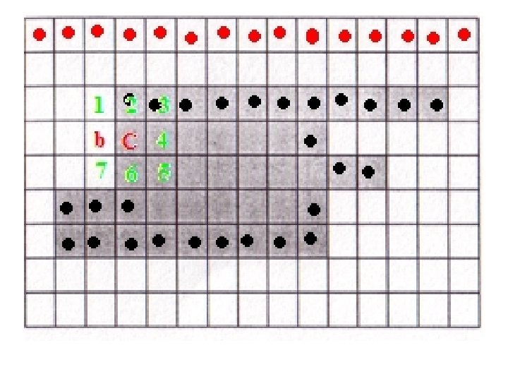
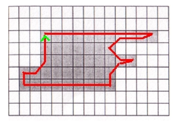
• Set C = ni and b = ni-1. Include C in B, the sequence of boundary pixels. • Repeat till you get C = X and b = b 0

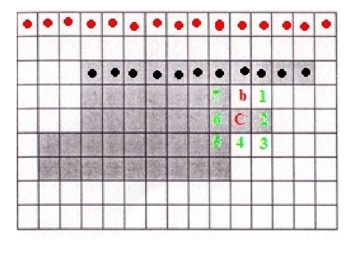
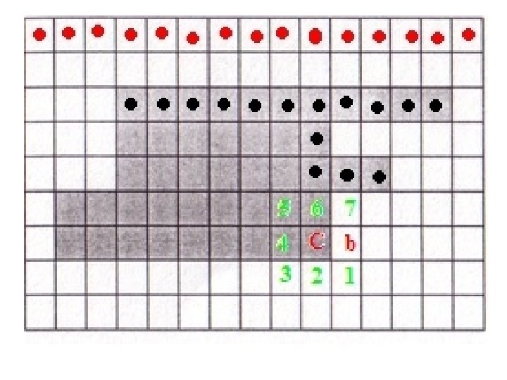
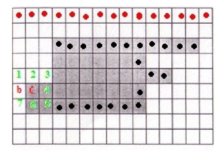
C = X, b = b 0 !!STOP!!

Chain codes • Assign a number to each direction: 4 connectivity 8 connectivity

Chain codes • Start from a point and proceed in a clockwise direction: • The chain code is: 07666664…. .

Chain code: Issues • Different starting point would obviously give a different chain code. • The chain code is: 1212076666…. • Choose the chain code that gives the minimum integer, in this case: 076666…. (start with seq with most 0 s)

Chain code: Issues • In any real image, chains would be very long, and any small disturbance in the boundary would yield a different chain code. • Solution: Sample the boundary

Rotation invariance in chain codes • Use the first difference of chain code: Number of direction changes in a counter-clockwise direction between adjacent elements of the chain code. • The chain code is 0766666453321212 • The first difference code is: 770000616077171

Boundary signatures • Distance from centroid vs. angle: • Will not work if the region is not star-shaped with respect to the centroid. • Is not invariant to scaling and rotation

Skeletons • Object region Graph • Based on Medial Axis transform [Harry Blum, 1967] • Given a boundary B, the locus of points in the entire region which have atleast two nearest neighbors in B is called the medial axis of B.

Descriptors • Length: Number of pixels on the boundary. • Diameter of the boundary B: • Shape numbers: Given a chain coded boundary, the shape number is defined as the first difference of smallest magnitude. • Order of shape number is the number of digits in its representation.

Fourier descriptors • Boundary: • Treat each element as a complex number: • Take the DFT:

Invariance of Fourier descriptors

Approximate Fourier descriptors • Set • Let

Approximate Fourier descriptors