DATA MINING LECTURE 4 Frequent Itemsets and Association

DATA MINING LECTURE 4 Frequent Itemsets and Association Rules

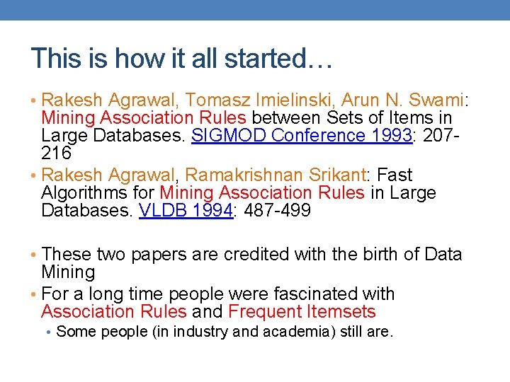
This is how it all started… • Rakesh Agrawal, Tomasz Imielinski, Arun N. Swami: Mining Association Rules between Sets of Items in Large Databases. SIGMOD Conference 1993: 207216 • Rakesh Agrawal, Ramakrishnan Srikant: Fast Algorithms for Mining Association Rules in Large Databases. VLDB 1994: 487 -499 • These two papers are credited with the birth of Data Mining • For a long time people were fascinated with Association Rules and Frequent Itemsets • Some people (in industry and academia) still are.

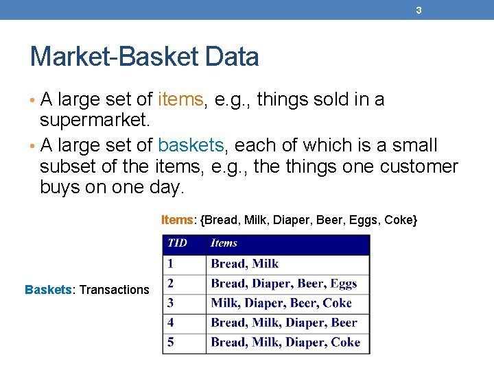
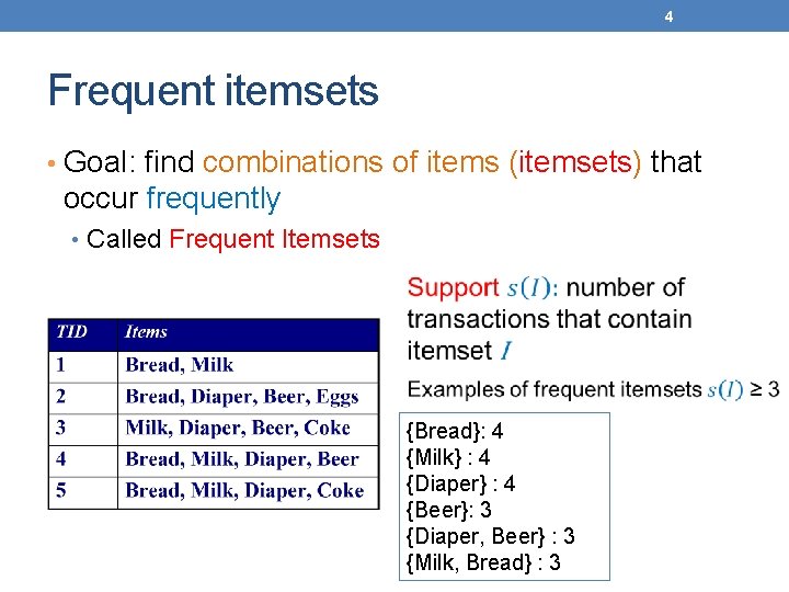
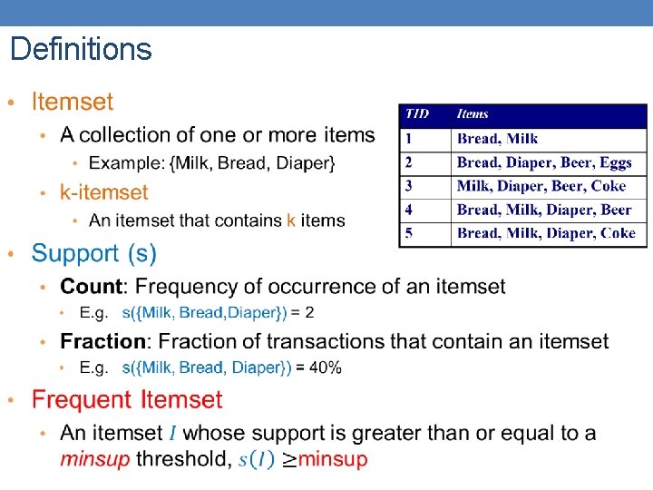
3 Market-Basket Data • A large set of items, e. g. , things sold in a supermarket. • A large set of baskets, each of which is a small subset of the items, e. g. , the things one customer buys on one day. Items: {Bread, Milk, Diaper, Beer, Eggs, Coke} Baskets: Transactions

4 Frequent itemsets • Goal: find combinations of items (itemsets) that occur frequently • Called Frequent Itemsets {Bread}: 4 {Milk} : 4 {Diaper} : 4 {Beer}: 3 {Diaper, Beer} : 3 {Milk, Bread} : 3

5 Market-Baskets – (2) • Really, a general many-to-many mapping (association) between two kinds of things, where the one (the baskets) is a set of the other (the items) • But we ask about connections among “items, ” not “baskets. ” • The technology focuses on common/frequent events, not rare events (“long tail”).

6 Applications – (1) • Items = products; baskets = sets of products someone bought in one trip to the store. • Example application: given that many people buy beer and diapers together: • Run a sale on diapers; raise price of beer. • Only useful if many buy diapers & beer.

7 Applications – (2) • Baskets = Web pages; items = words. • Example application: Unusual words appearing together in a large number of documents, e. g. , “Brad” and “Angelina, ” may indicate an interesting relationship.

8 Applications – (3) • Baskets = sentences; items = documents containing those sentences. • Example application: Items that appear together too often could represent plagiarism. • Notice items do not have to be “in” baskets.

Definitions •

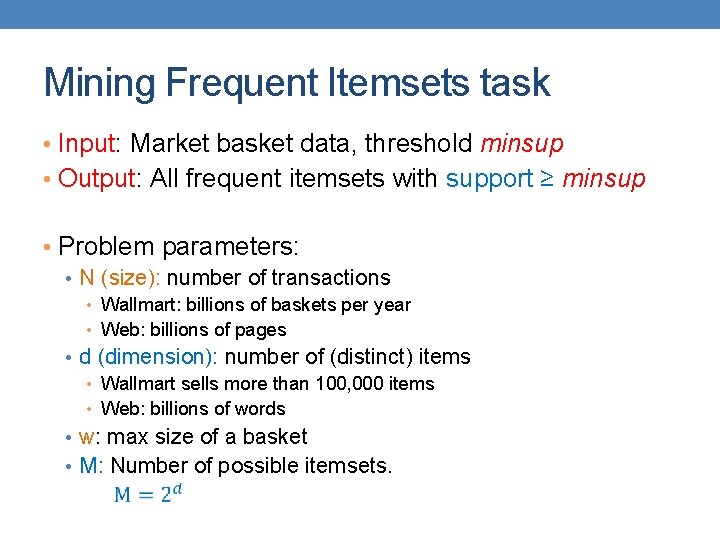
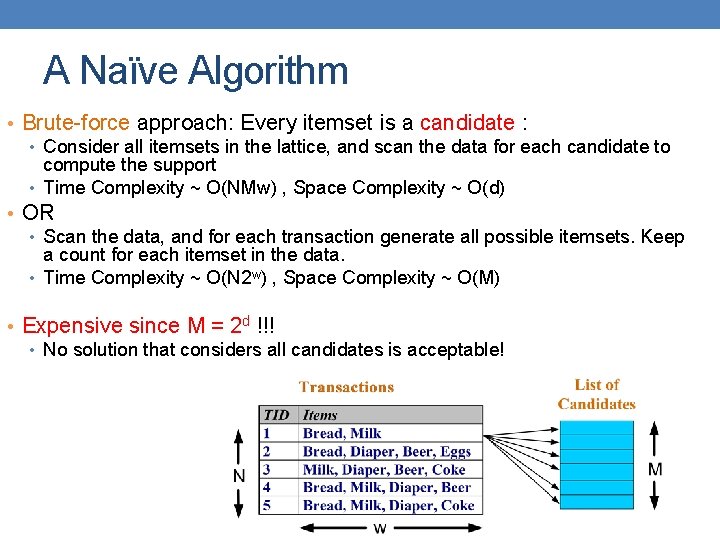
Mining Frequent Itemsets task • Input: Market basket data, threshold minsup • Output: All frequent itemsets with support ≥ minsup • Problem parameters: • N (size): number of transactions • Wallmart: billions of baskets per year • Web: billions of pages • d (dimension): number of (distinct) items • Wallmart sells more than 100, 000 items • Web: billions of words • w: max size of a basket • M: Number of possible itemsets.

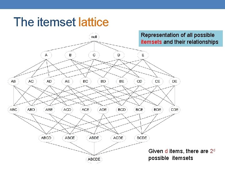
The itemset lattice Representation of all possible itemsets and their relationships Given d items, there are 2 d possible itemsets

A Naïve Algorithm • Brute-force approach: Every itemset is a candidate : • Consider all itemsets in the lattice, and scan the data for each candidate to compute the support • Time Complexity ~ O(NMw) , Space Complexity ~ O(d) • OR • Scan the data, and for each transaction generate all possible itemsets. Keep a count for each itemset in the data. • Time Complexity ~ O(N 2 w) , Space Complexity ~ O(M) • Expensive since M = 2 d !!! • No solution that considers all candidates is acceptable!

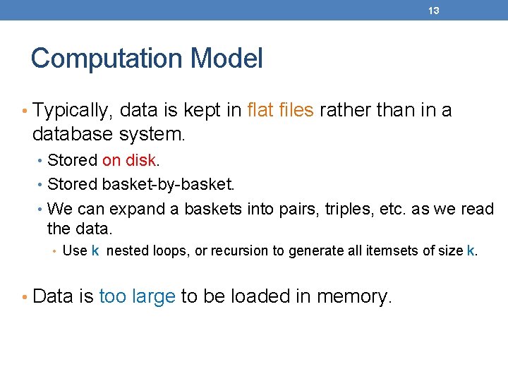
13 Computation Model • Typically, data is kept in flat files rather than in a database system. • Stored on disk. • Stored basket-by-basket. • We can expand a baskets into pairs, triples, etc. as we read the data. • Use k nested loops, or recursion to generate all itemsets of size k. • Data is too large to be loaded in memory.

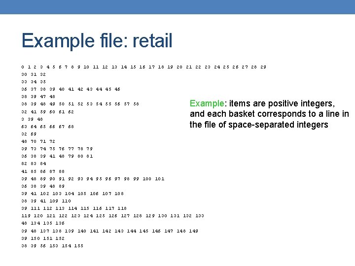
Example file: retail 0 1 2 3 4 5 6 7 8 9 10 11 12 13 14 15 16 17 18 19 20 21 22 23 24 25 26 27 28 29 30 31 32 33 34 35 36 37 38 39 40 41 42 43 44 45 46 38 39 47 48 38 39 48 49 50 51 52 53 54 55 56 57 58 32 41 59 60 61 62 3 39 48 63 64 65 66 67 68 32 69 48 70 71 72 39 73 74 75 76 77 78 79 36 38 39 41 48 79 80 81 82 83 84 41 85 86 87 88 39 48 89 90 91 92 93 94 95 96 97 98 99 100 101 36 38 39 48 89 39 41 102 103 104 105 106 107 108 38 39 41 109 110 39 111 112 113 114 115 116 117 118 119 120 121 122 123 124 125 126 127 128 129 130 131 132 133 48 134 135 136 39 48 137 138 139 140 141 142 143 144 145 146 147 148 149 39 150 151 152 38 39 56 153 154 155 Example: items are positive integers, and each basket corresponds to a line in the file of space-separated integers

15 Computation Model – (2) • The true cost of mining disk-resident data is usually the number of disk I/O’s. • In practice, association-rule algorithms read the data in passes – all baskets read in turn. • Thus, we measure the cost by the number of passes an algorithm takes.

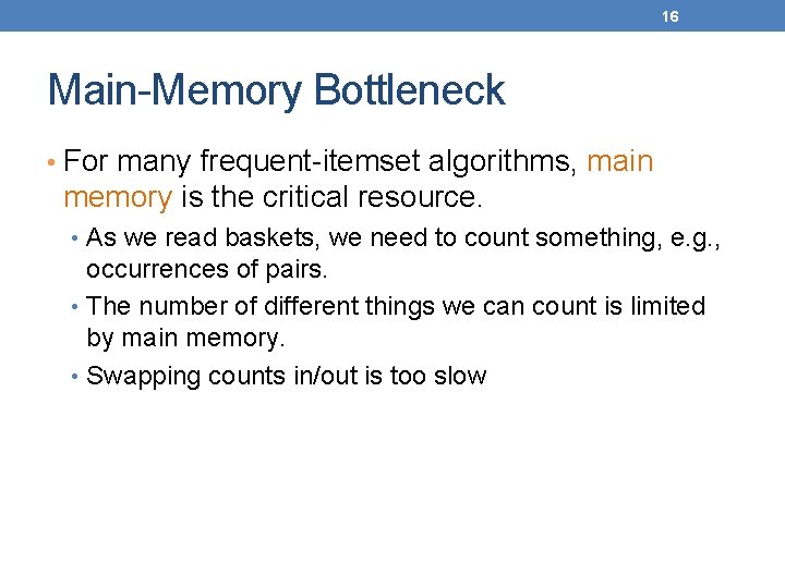
16 Main-Memory Bottleneck • For many frequent-itemset algorithms, main memory is the critical resource. • As we read baskets, we need to count something, e. g. , occurrences of pairs. • The number of different things we can count is limited by main memory. • Swapping counts in/out is too slow

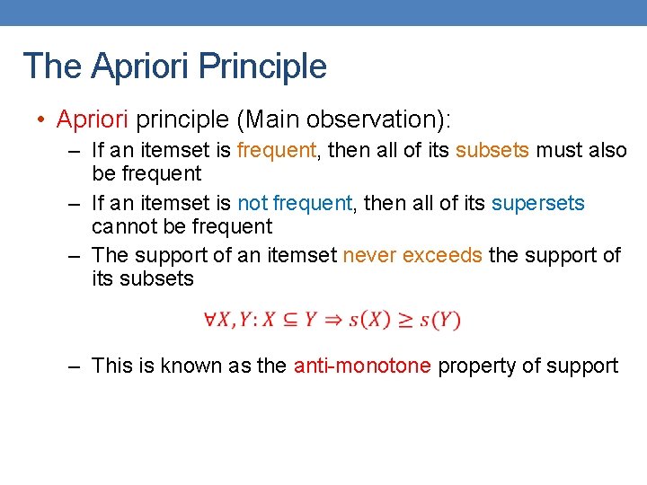
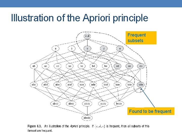
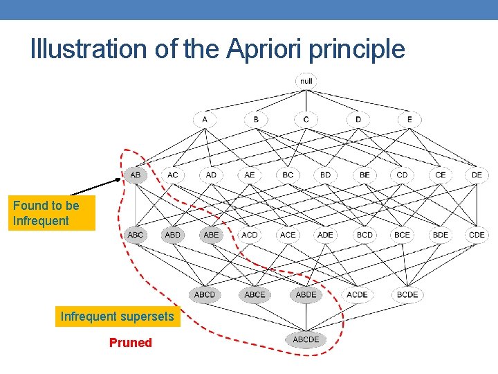
The Apriori Principle • Apriori principle (Main observation): – If an itemset is frequent, then all of its subsets must also be frequent – If an itemset is not frequent, then all of its supersets cannot be frequent – The support of an itemset never exceeds the support of its subsets – This is known as the anti-monotone property of support

Illustration of the Apriori principle Frequent subsets Found to be frequent

Illustration of the Apriori principle Found to be Infrequent supersets Pruned

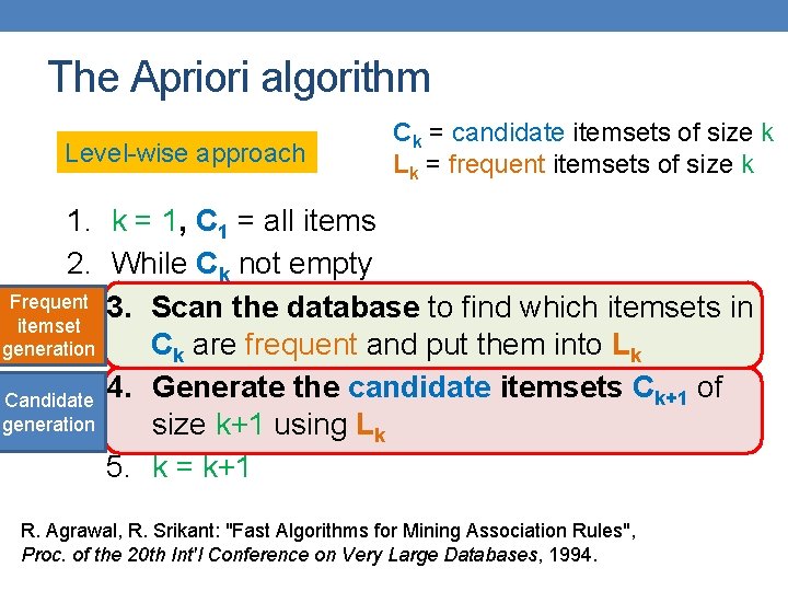
The Apriori algorithm Level-wise approach Ck = candidate itemsets of size k Lk = frequent itemsets of size k 1. k = 1, C 1 = all items 2. While Ck not empty Frequent 3. Scan the database to find which itemsets in itemset Ck are frequent and put them into Lk generation Candidate 4. Generate the candidate itemsets Ck+1 of generation size k+1 using Lk 5. k = k+1 R. Agrawal, R. Srikant: "Fast Algorithms for Mining Association Rules", Proc. of the 20 th Int'l Conference on Very Large Databases, 1994.

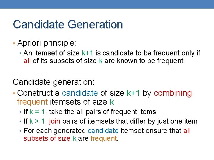
Candidate Generation • Apriori principle: • An itemset of size k+1 is candidate to be frequent only if all of its subsets of size k are known to be frequent Candidate generation: • Construct a candidate of size k+1 by combining frequent itemsets of size k • If k = 1, take the all pairs of frequent items • If k > 1, join pairs of itemsets that differ by just one item • For each generated candidate itemset ensure that all subsets of size k are frequent.

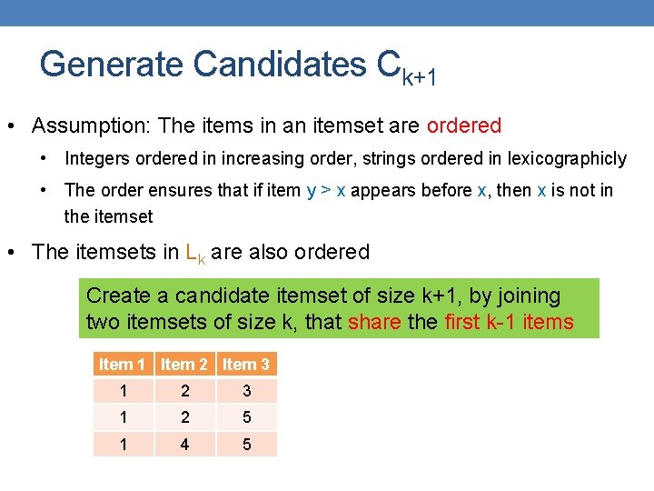
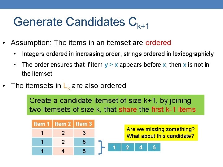
Generate Candidates Ck+1 • Assumption: The items in an itemset are ordered • Integers ordered in increasing order, strings ordered in lexicographicly • The order ensures that if item y > x appears before x, then x is not in the itemset • The itemsets in Lk are also ordered Create a candidate itemset of size k+1, by joining two itemsets of size k, that share the first k-1 items Item 1 Item 2 Item 3 1 2 5 1 4 5

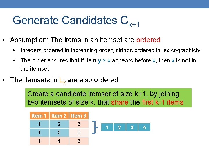
Generate Candidates Ck+1 • Assumption: The items in an itemset are ordered • Integers ordered in increasing order, strings ordered in lexicographicly • The order ensures that if item y > x appears before x, then x is not in the itemset • The itemsets in Lk are also ordered Create a candidate itemset of size k+1, by joining two itemsets of size k, that share the first k-1 items Item 1 Item 2 Item 3 1 2 5 1 4 5 1 2 3 5

Generate Candidates Ck+1 • Assumption: The items in an itemset are ordered • Integers ordered in increasing order, strings ordered in lexicographicly • The order ensures that if item y > x appears before x, then x is not in the itemset • The itemsets in Lk are also ordered Create a candidate itemset of size k+1, by joining two itemsets of size k, that share the first k-1 items Item 1 Item 2 Item 3 1 2 5 1 4 5 Are we missing something? What about this candidate? 1 2 4 5

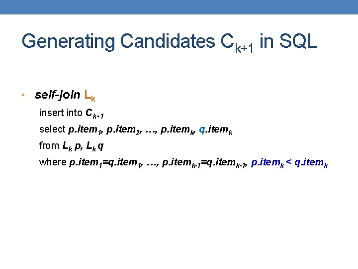
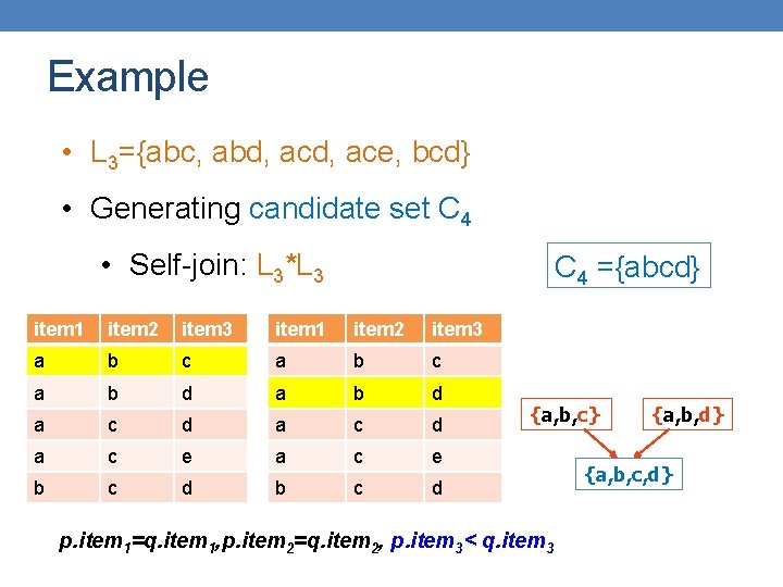
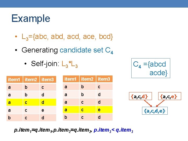
Generating Candidates Ck+1 in SQL • self-join Lk insert into Ck+1 select p. item 1, p. item 2, …, p. itemk, q. itemk from Lk p, Lk q where p. item 1=q. item 1, …, p. itemk-1=q. itemk-1, p. itemk < q. itemk

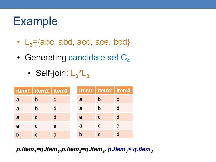
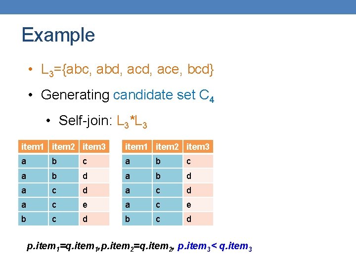
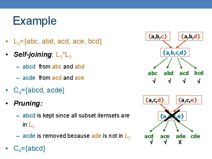
Example • L 3={abc, abd, ace, bcd} • Generating candidate set C 4 • Self-join: L 3*L 3 item 1 item 2 item 3 a b c a b d a c e b c d p. item 1=q. item 1, p. item 2=q. item 2, p. item 3< q. item 3

Example • L 3={abc, abd, ace, bcd} • Generating candidate set C 4 • Self-join: L 3*L 3 item 1 item 2 item 3 a b c a b d a c e b c d p. item 1=q. item 1, p. item 2=q. item 2, p. item 3< q. item 3

Example • L 3={abc, abd, ace, bcd} • Generating candidate set C 4 • Self-join: L 3*L 3 C 4 ={abcd} item 1 item 2 item 3 a b c a b d a c e b c d {a, b, c} p. item 1=q. item 1, p. item 2=q. item 2, p. item 3< q. item 3 {a, b, d} {a, b, c, d}

Example • L 3={abc, abd, ace, bcd} • Generating candidate set C 4 • Self-join: L 3*L 3 item 1 item 2 item 3 a b c a b d a c e b c d C 4 ={abcd acde} {a, c, d} p. item 1=q. item 1, p. item 2=q. item 2, p. item 3< q. item 3 {a, c, e} {a, c, d, e}

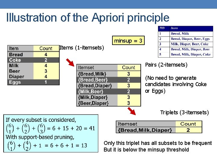
Illustration of the Apriori principle minsup = 3 Items (1 -itemsets) Pairs (2 -itemsets) (No need to generate candidates involving Coke or Eggs) Triplets (3 -itemsets) Only this triplet has all subsets to be frequent But it is below the minsup threshold

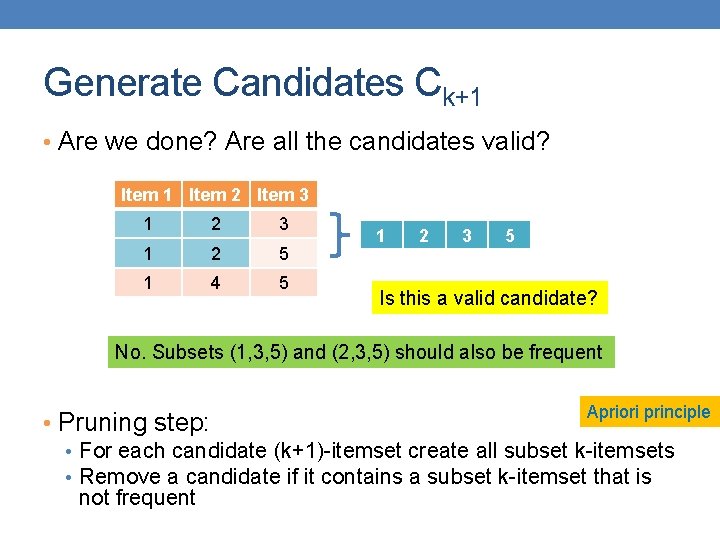
Generate Candidates Ck+1 • Are we done? Are all the candidates valid? Item 1 Item 2 Item 3 1 2 5 1 4 5 1 2 3 5 Is this a valid candidate? No. Subsets (1, 3, 5) and (2, 3, 5) should also be frequent Apriori principle • Pruning step: • For each candidate (k+1)-itemset create all subset k-itemsets • Remove a candidate if it contains a subset k-itemset that is not frequent

Example • L 3={abc, abd, ace, bcd} {a, b, c, d} • Self-joining: L 3*L 3 – abcd from abc and abd – acde from acd and ace {a, b, d} abc abd acd bcd • C 4={abcd, acde} • Pruning: {a, c, d} – abcd is kept since all subset itemsets are {a, c, e} {a, c, d, e} in L 3 – acde is removed because ade is not in L 3 • C 4={abcd} acd ace ade cde X

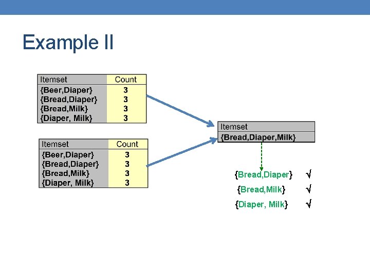
Example II {Bread, Diaper} {Bread, Milk} {Diaper, Milk}

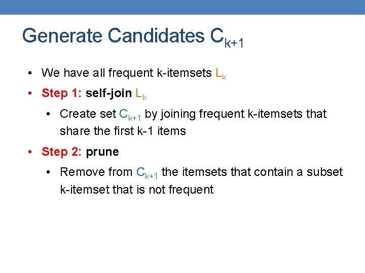
Generate Candidates Ck+1 • We have all frequent k-itemsets Lk • Step 1: self-join Lk • Create set Ck+1 by joining frequent k-itemsets that share the first k-1 items • Step 2: prune • Remove from Ck+1 the itemsets that contain a subset k-itemset that is not frequent

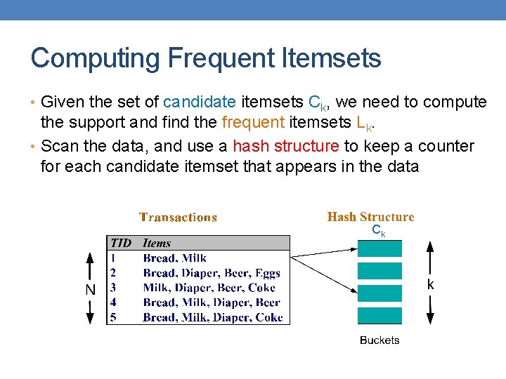
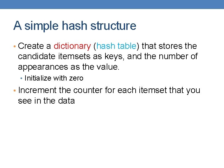
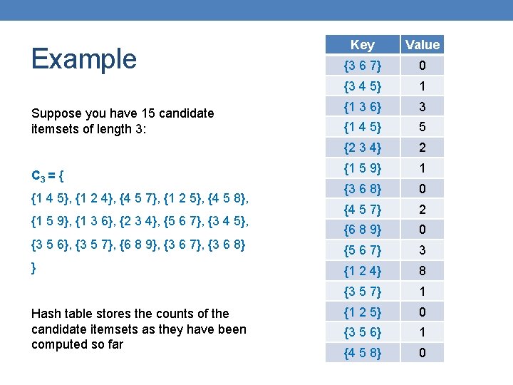
Computing Frequent Itemsets • Given the set of candidate itemsets Ck, we need to compute the support and find the frequent itemsets Lk. • Scan the data, and use a hash structure to keep a counter for each candidate itemset that appears in the data Ck

A simple hash structure • Create a dictionary (hash table) that stores the candidate itemsets as keys, and the number of appearances as the value. • Initialize with zero • Increment the counter for each itemset that you see in the data

Key Value {3 6 7} 0 {3 4 5} 1 {1 3 6} 3 {1 4 5} 5 {2 3 4} 2 {1 5 9} 1 {3 6 8} 0 {4 5 7} 2 {6 8 9} 0 {3 5 6}, {3 5 7}, {6 8 9}, {3 6 7}, {3 6 8} {5 6 7} 3 } {1 2 4} 8 {3 5 7} 1 {1 2 5} 0 {3 5 6} 1 {4 5 8} 0 Example Suppose you have 15 candidate itemsets of length 3: C 3 = { {1 4 5}, {1 2 4}, {4 5 7}, {1 2 5}, {4 5 8}, {1 5 9}, {1 3 6}, {2 3 4}, {5 6 7}, {3 4 5}, Hash table stores the counts of the candidate itemsets as they have been computed so far

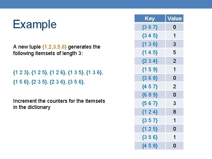
Example A new tuple {1, 2, 3, 5, 6} generates the following itemsets of length 3: {1 2 3}, {1 2 5}, {1 2 6}, {1 3 5}, {1 3 6}, {1 5 6}, {2 3 5}, {2 3 6}, {3 5 6}, Increment the counters for the itemsets in the dictionary Key Value {3 6 7} 0 {3 4 5} 1 {1 3 6} 3 {1 4 5} 5 {2 3 4} 2 {1 5 9} 1 {3 6 8} 0 {4 5 7} 2 {6 8 9} 0 {5 6 7} 3 {1 2 4} 8 {3 5 7} 1 {1 2 5} 0 {3 5 6} 1 {4 5 8} 0

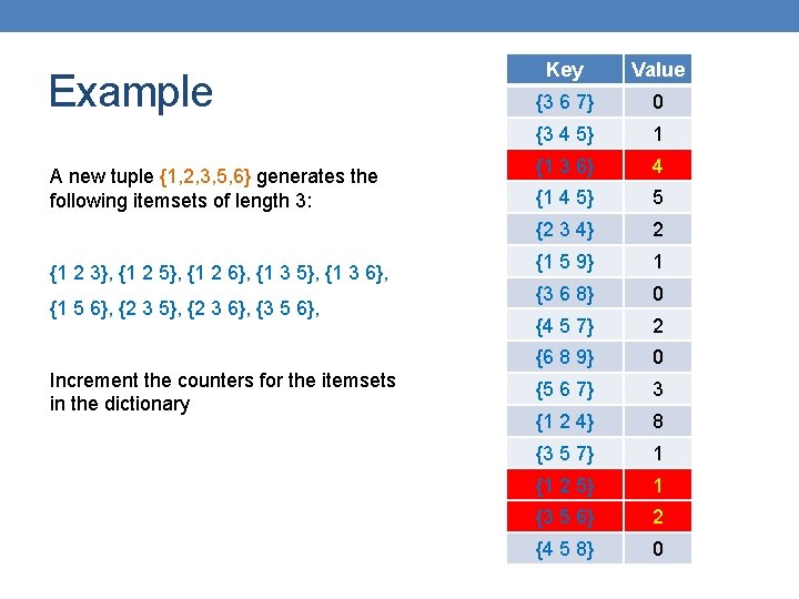
Example A new tuple {1, 2, 3, 5, 6} generates the following itemsets of length 3: {1 2 3}, {1 2 5}, {1 2 6}, {1 3 5}, {1 3 6}, {1 5 6}, {2 3 5}, {2 3 6}, {3 5 6}, Increment the counters for the itemsets in the dictionary Key Value {3 6 7} 0 {3 4 5} 1 {1 3 6} 4 {1 4 5} 5 {2 3 4} 2 {1 5 9} 1 {3 6 8} 0 {4 5 7} 2 {6 8 9} 0 {5 6 7} 3 {1 2 4} 8 {3 5 7} 1 {1 2 5} 1 {3 5 6} 2 {4 5 8} 0

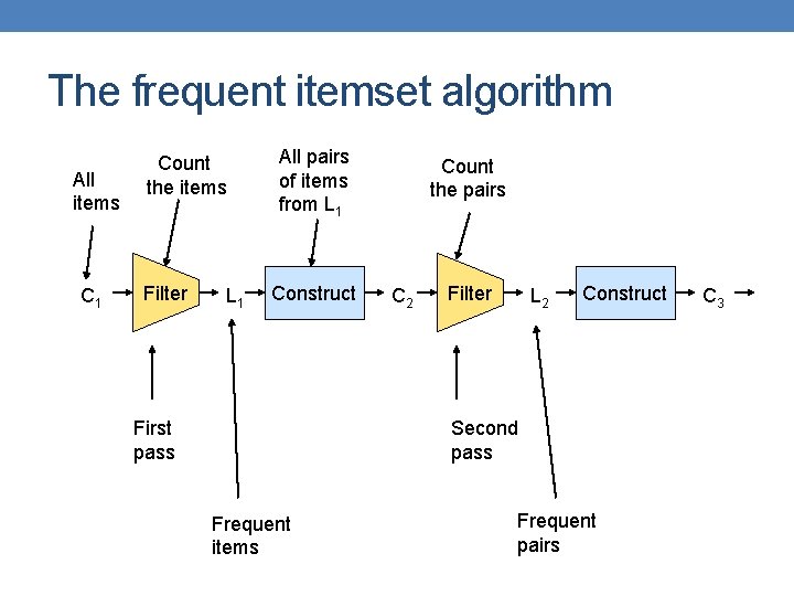
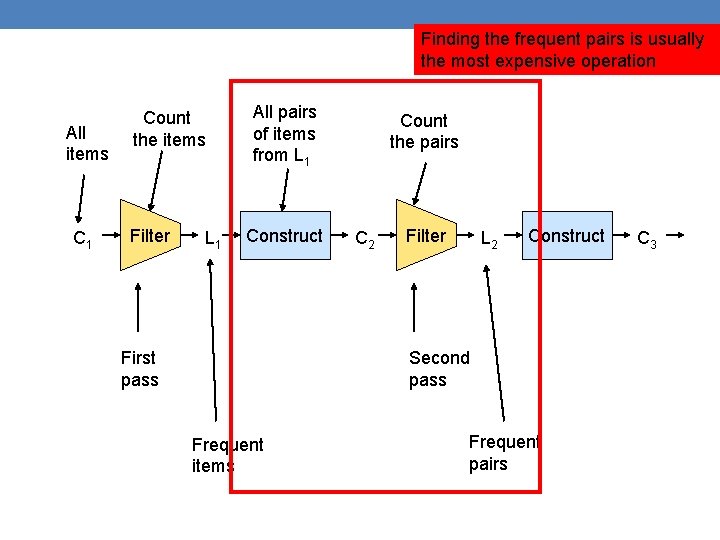
The frequent itemset algorithm All items C 1 Count the items Filter L 1 All pairs of items from L 1 Construct First pass Count the pairs C 2 Filter L 2 Construct Second pass Frequent items Frequent pairs C 3

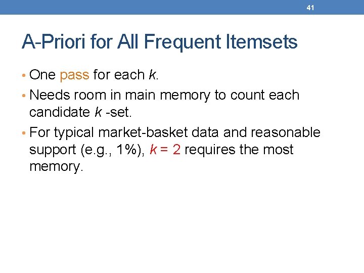
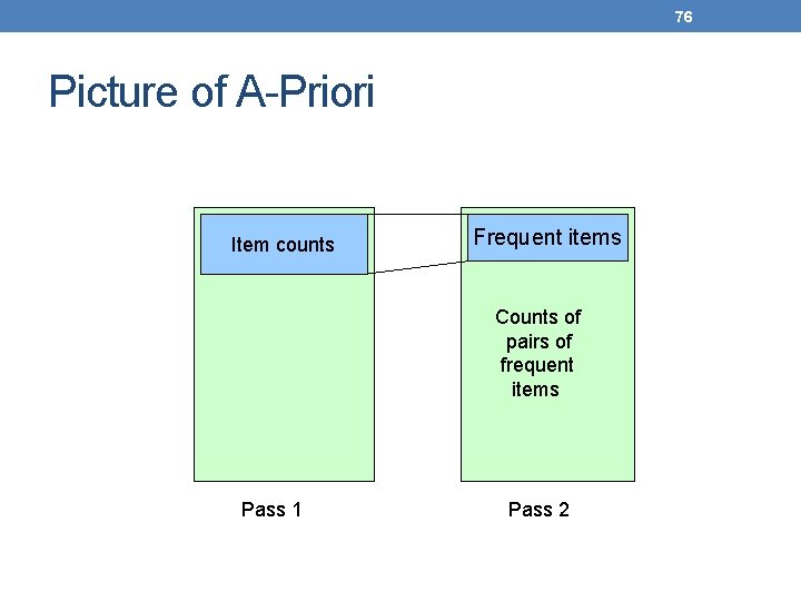
41 A-Priori for All Frequent Itemsets • One pass for each k. • Needs room in main memory to count each candidate k -set. • For typical market-basket data and reasonable support (e. g. , 1%), k = 2 requires the most memory.

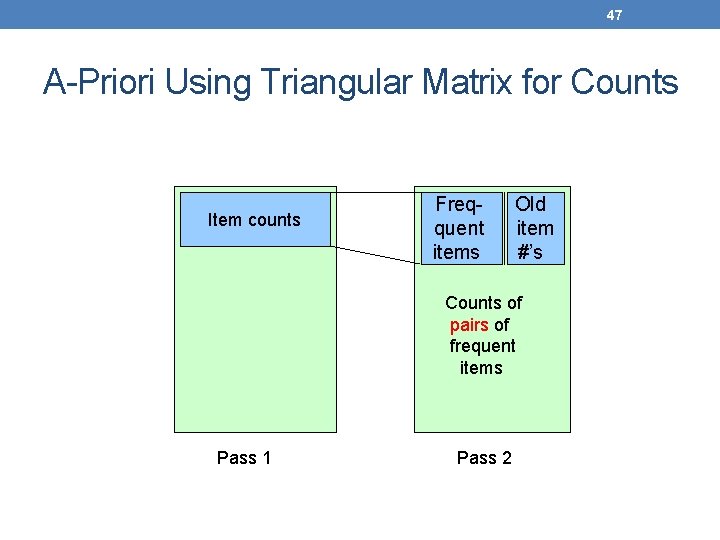
42 Picture of A-Priori Item counts Frequent items Counts of pairs of frequent items Pass 1 Pass 2

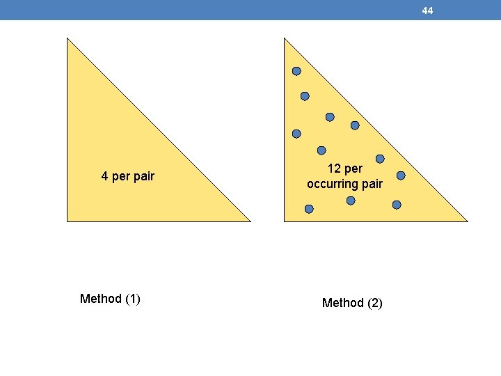
43 Details of Main-Memory Counting • Two approaches: 1. Count all pairs, using a “triangular matrix” = one dimensional array that stores the lower diagonal. 2. Keep a table of triples [i, j, c] = “the count of the pair of items {i, j } is c. ” • (1) requires only 4 bytes/pair. • Note: always assume integers are 4 bytes. • (2) requires 12 bytes/pair, but only for those pairs with count > 0.

44 4 per pair Method (1) 12 per occurring pair Method (2)

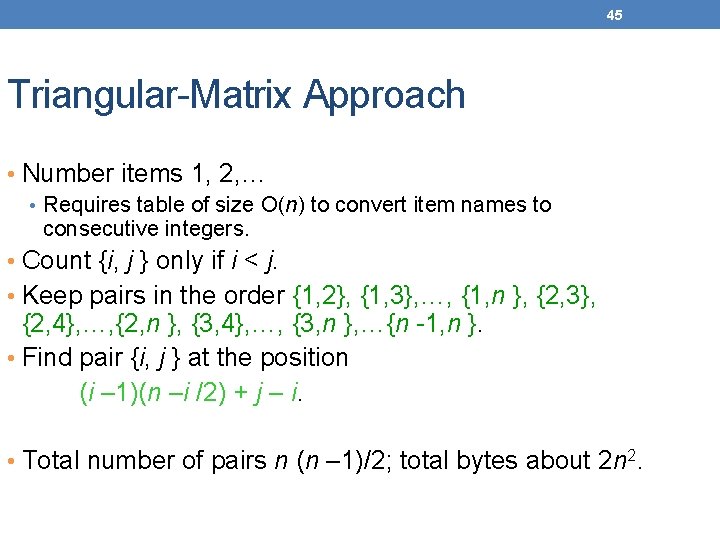
45 Triangular-Matrix Approach • Number items 1, 2, … • Requires table of size O(n) to convert item names to consecutive integers. • Count {i, j } only if i < j. • Keep pairs in the order {1, 2}, {1, 3}, …, {1, n }, {2, 3}, {2, 4}, …, {2, n }, {3, 4}, …, {3, n }, …{n -1, n }. • Find pair {i, j } at the position (i – 1)(n –i /2) + j – i. • Total number of pairs n (n – 1)/2; total bytes about 2 n 2.

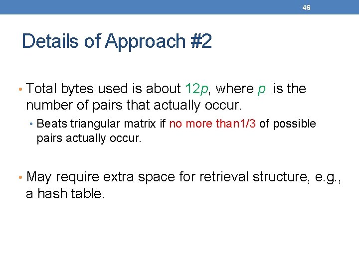
46 Details of Approach #2 • Total bytes used is about 12 p, where p is the number of pairs that actually occur. • Beats triangular matrix if no more than 1/3 of possible pairs actually occur. • May require extra space for retrieval structure, e. g. , a hash table.

47 A-Priori Using Triangular Matrix for Counts Item counts Freqquent items Old item #’s Counts of pairs of frequent items Pass 1 Pass 2

ASSOCIATION RULES

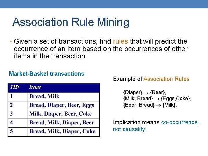
Association Rule Mining • Given a set of transactions, find rules that will predict the occurrence of an item based on the occurrences of other items in the transaction Market-Basket transactions Example of Association Rules {Diaper} {Beer}, {Milk, Bread} {Eggs, Coke}, {Beer, Bread} {Milk}, Implication means co-occurrence, not causality!

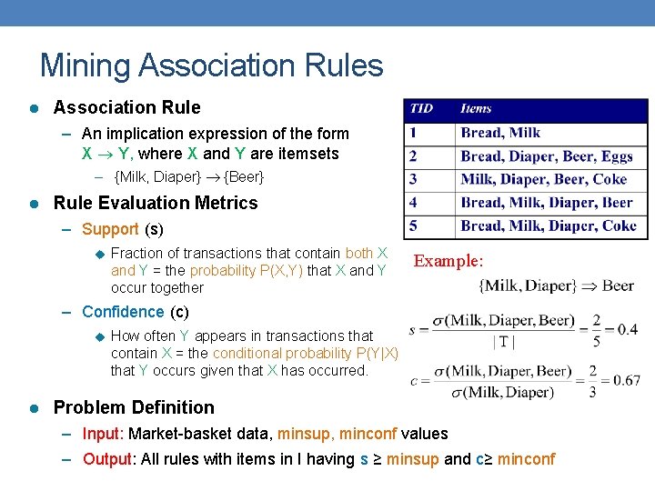
Mining Association Rules l Association Rule – An implication expression of the form X Y, where X and Y are itemsets – {Milk, Diaper} {Beer} l Rule Evaluation Metrics – Support (s) u Fraction of transactions that contain both X and Y = the probability P(X, Y) that X and Y occur together Example: – Confidence (c) u l How often Y appears in transactions that contain X = the conditional probability P(Y|X) that Y occurs given that X has occurred. Problem Definition – Input: Market-basket data, minsup, minconf values – Output: All rules with items in I having s ≥ minsup and c≥ minconf

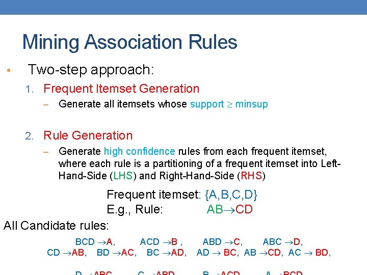
Mining Association Rules • Two-step approach: 1. Frequent Itemset Generation – Generate all itemsets whose support minsup 2. Rule Generation – Generate high confidence rules from each frequent itemset, where each rule is a partitioning of a frequent itemset into Left. Hand-Side (LHS) and Right-Hand-Side (RHS) Frequent itemset: {A, B, C, D} E. g. , Rule: AB CD All Candidate rules: BCD A, ACD B , CD AB, BD AC, BC AD, ABD C, ABC D, AD BC, AB CD, AC BD,

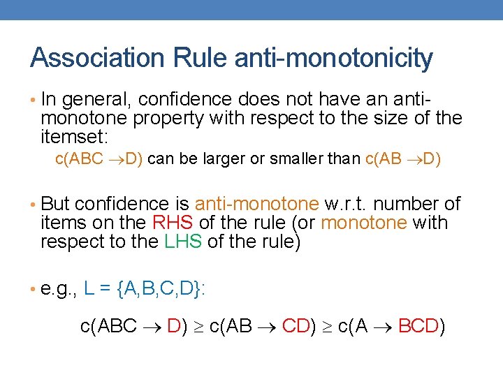
Association Rule anti-monotonicity • In general, confidence does not have an anti- monotone property with respect to the size of the itemset: c(ABC D) can be larger or smaller than c(AB D) • But confidence is anti-monotone w. r. t. number of items on the RHS of the rule (or monotone with respect to the LHS of the rule) • e. g. , L = {A, B, C, D}: c(ABC D) c(AB CD) c(A BCD)

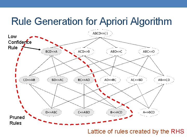
Rule Generation for Apriori Algorithm Low Confidence Rule Pruned Rules Lattice of rules created by the RHS

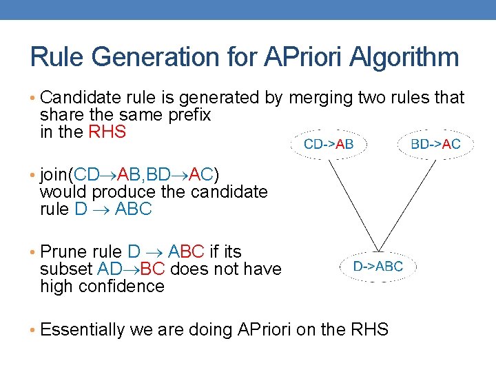
Rule Generation for APriori Algorithm • Candidate rule is generated by merging two rules that share the same prefix in the RHS • join(CD AB, BD AC) would produce the candidate rule D ABC • Prune rule D ABC if its subset AD BC does not have high confidence • Essentially we are doing APriori on the RHS

RESULT POST-PROCESSING

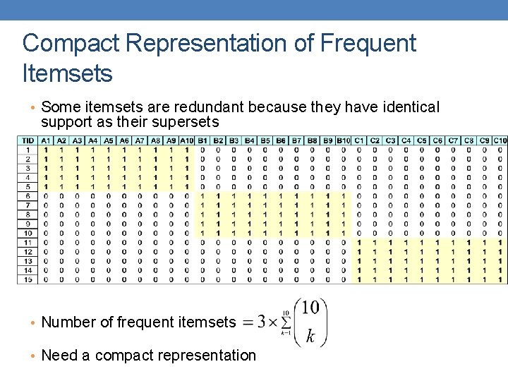
Compact Representation of Frequent Itemsets • Some itemsets are redundant because they have identical support as their supersets • Number of frequent itemsets • Need a compact representation

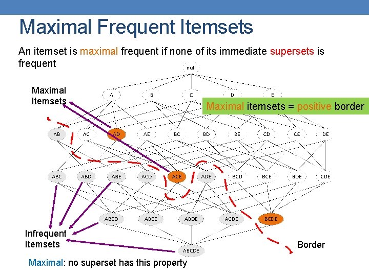
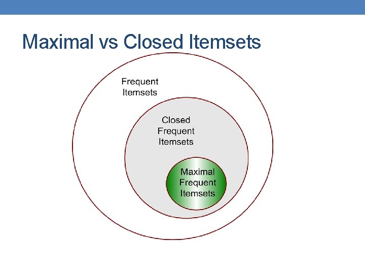
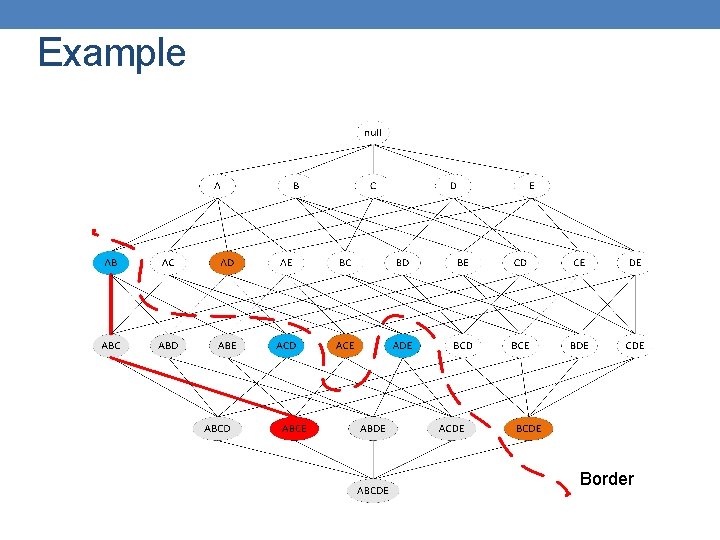
Maximal Frequent Itemsets An itemset is maximal frequent if none of its immediate supersets is frequent Maximal Itemsets Infrequent Itemsets Maximal: no superset has this property Maximal itemsets = positive border Border

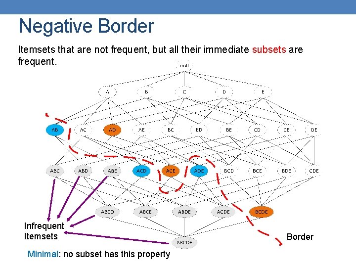
Negative Border Itemsets that are not frequent, but all their immediate subsets are frequent. Infrequent Itemsets Minimal: no subset has this property Border

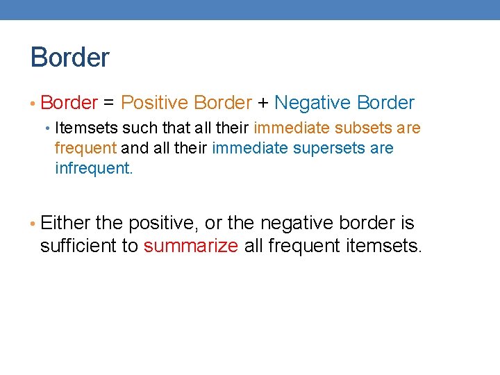
Border • Border = Positive Border + Negative Border • Itemsets such that all their immediate subsets are frequent and all their immediate supersets are infrequent. • Either the positive, or the negative border is sufficient to summarize all frequent itemsets.

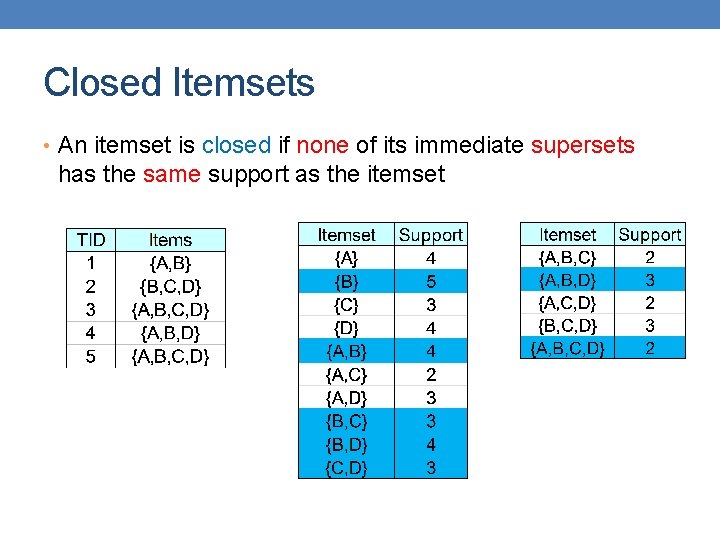
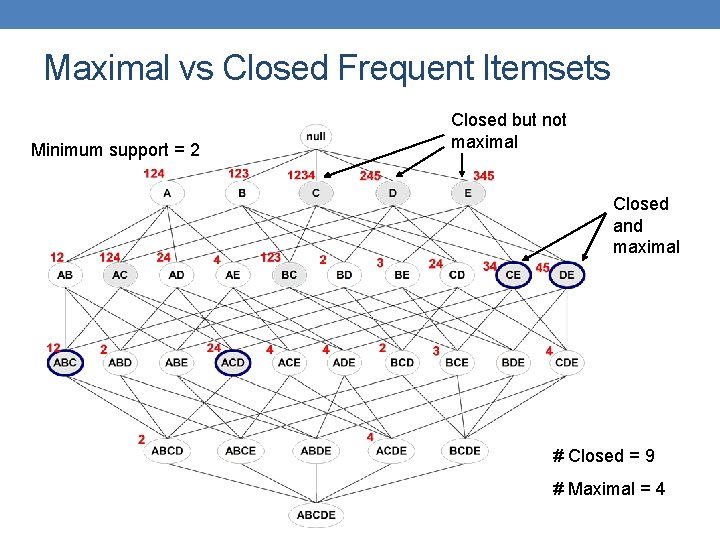
Closed Itemsets • An itemset is closed if none of its immediate supersets has the same support as the itemset

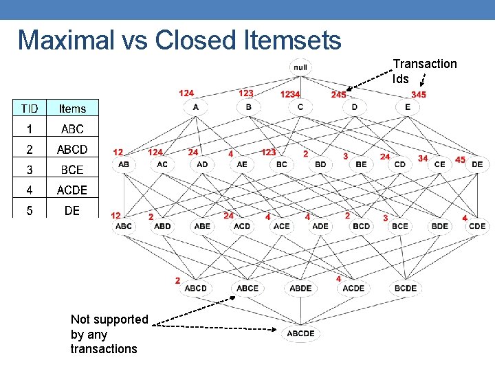
Maximal vs Closed Itemsets Transaction Ids Not supported by any transactions

Maximal vs Closed Frequent Itemsets Minimum support = 2 Closed but not maximal Closed and maximal # Closed = 9 # Maximal = 4

Maximal vs Closed Itemsets

Pattern Evaluation • Association rule algorithms tend to produce too many rules but many of them are uninteresting or redundant • Redundant if {A, B, C} {D} and {A, B} {D} have same support & confidence • Summarization techniques • Uninteresting, if the pattern that is revealed does not offer useful information. • Interestingness measures: a hard problem to define • Interestingness measures can be used to prune/rank the derived patterns • Subjective measures: require human analyst • Objective measures: rely on the data. • In the original formulation of association rules, support & confidence are the only measures used

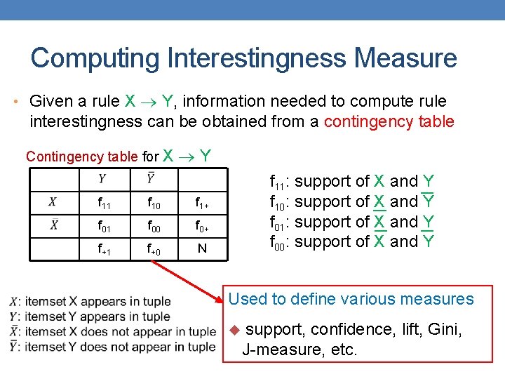
Computing Interestingness Measure • Given a rule X Y, information needed to compute rule interestingness can be obtained from a contingency table Contingency table for X Y f 11 f 10 f 1+ f 01 f 00 f 0+ f+1 f+0 N f 11: support of X and Y f 10: support of X and Y f 01: support of X and Y f 00: support of X and Y Used to define various measures u support, confidence, lift, Gini, J-measure, etc.

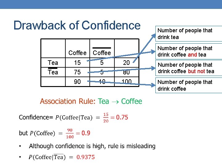
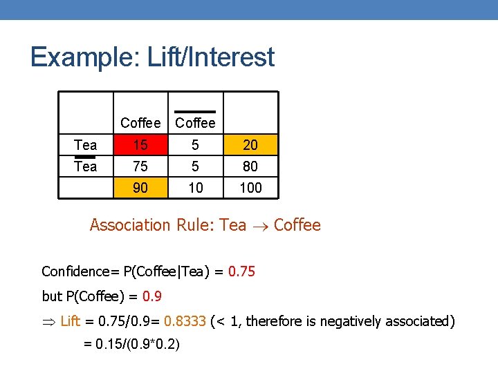
Drawback of Confidence Number of people that drink tea Number of people that drink coffee and tea Coffee Tea 15 5 20 Tea 75 5 80 90 10 100 Number of people that drink coffee but not tea Number of people that drink coffee

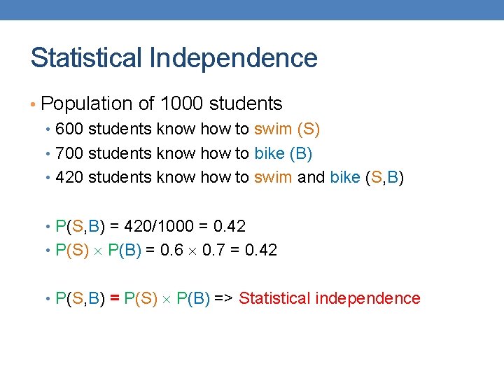
Statistical Independence • Population of 1000 students • 600 students know how to swim (S) • 700 students know how to bike (B) • 420 students know how to swim and bike (S, B) • P(S, B) = 420/1000 = 0. 42 • P(S) P(B) = 0. 6 0. 7 = 0. 42 • P(S, B) = P(S) P(B) => Statistical independence

Statistical Independence • Population of 1000 students • 600 students know how to swim (S) • 700 students know how to bike (B) • 500 students know how to swim and bike (S, B) • P(S, B) = 500/1000 = 0. 5 • P(S) P(B) = 0. 6 0. 7 = 0. 42 • P(S, B) > P(S) P(B) => Positively correlated

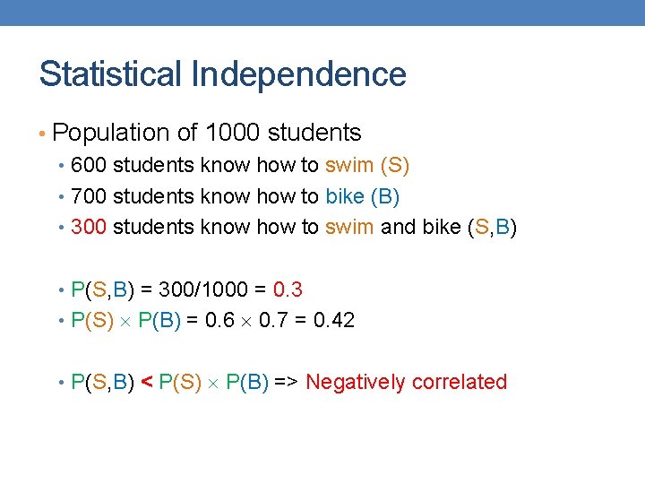
Statistical Independence • Population of 1000 students • 600 students know how to swim (S) • 700 students know how to bike (B) • 300 students know how to swim and bike (S, B) • P(S, B) = 300/1000 = 0. 3 • P(S) P(B) = 0. 6 0. 7 = 0. 42 • P(S, B) < P(S) P(B) => Negatively correlated

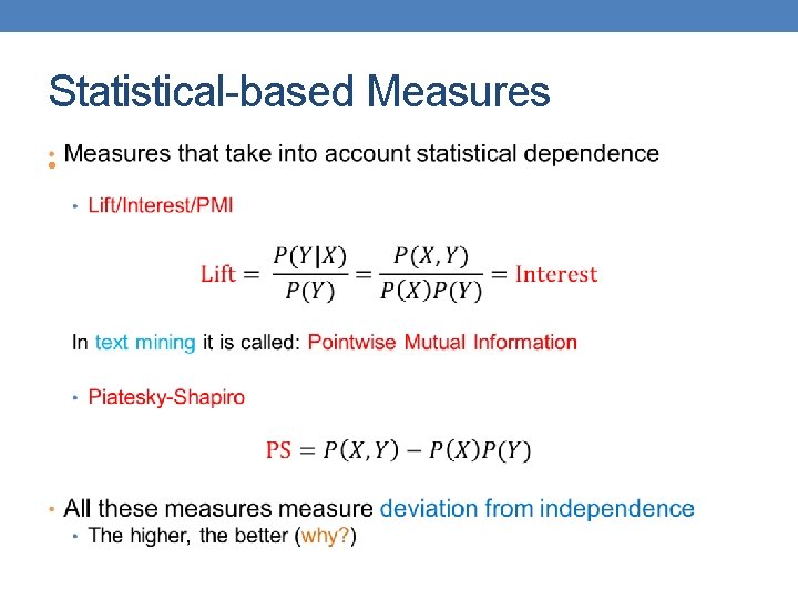
Statistical-based Measures •

Example: Lift/Interest Coffee Tea 15 5 20 Tea 75 5 80 90 10 100 Association Rule: Tea Coffee Confidence= P(Coffee|Tea) = 0. 75 but P(Coffee) = 0. 9 Þ Lift = 0. 75/0. 9= 0. 8333 (< 1, therefore is negatively associated) = 0. 15/(0. 9*0. 2)

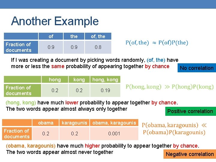
Another Example Fraction of documents of the of, the 0. 9 0. 8 If I was creating a document by picking words randomly, (of, the) have more or less the same probability of appearing together by chance No correlation hong kong hong, kong 0. 2 0. 19 Fraction of documents (hong, kong) have much lower probability to appear together by chance. The two words appear almost always only together Positive correlation Fraction of documents obama karagounis obama, karagounis 0. 2 0. 001 (obama, karagounis) have much higher probability to appear together by chance. The two words appear almost never together Negative correlation

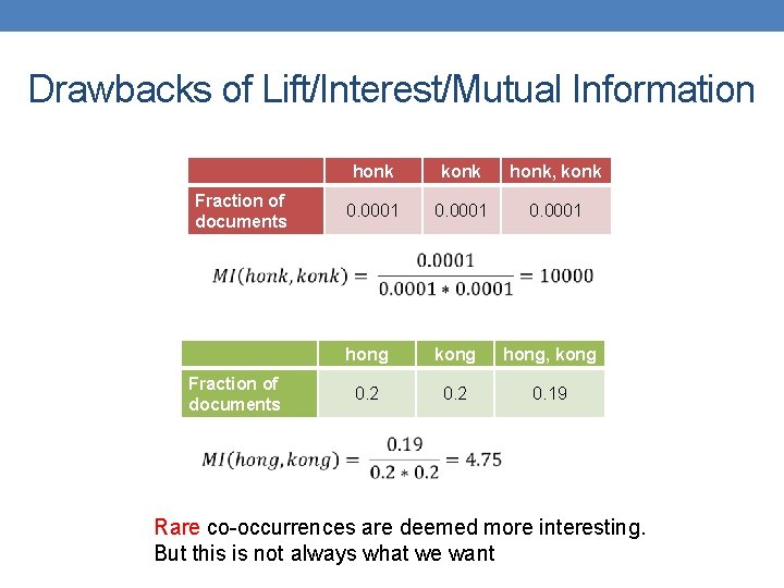
Drawbacks of Lift/Interest/Mutual Information Fraction of documents honk konk honk, konk 0. 0001 hong kong hong, kong 0. 2 0. 19 Rare co-occurrences are deemed more interesting. But this is not always what we want

ALTERNATIVE FREQUENT ITEMSET COMPUTATION Slides taken from Mining Massive Datasets course by Anand Rajaraman and Jeff Ullman.

Finding the frequent pairs is usually the most expensive operation All items C 1 Count the items Filter L 1 All pairs of items from L 1 Construct First pass Count the pairs C 2 Filter L 2 Construct Second pass Frequent items Frequent pairs C 3

76 Picture of A-Priori Item counts Frequent items Counts of pairs of frequent items Pass 1 Pass 2

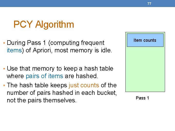
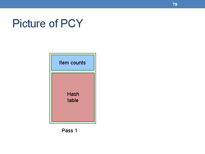
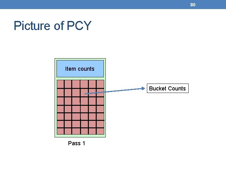
77 PCY Algorithm • During Pass 1 (computing frequent Item counts items) of Apriori, most memory is idle. • Use that memory to keep a hash table where pairs of items are hashed. • The hash table keeps just counts of the number of pairs hashed in each bucket, not the pairs themselves. Pass 1

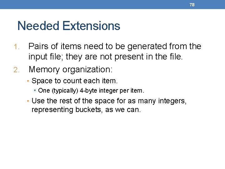
78 Needed Extensions Pairs of items need to be generated from the input file; they are not present in the file. 2. Memory organization: 1. • Space to count each item. • One (typically) 4 -byte integer per item. • Use the rest of the space for as many integers, representing buckets, as we can.

79 Picture of PCY Item counts Hash table Pass 1

80 Picture of PCY Item counts Bucket Counts Pass 1

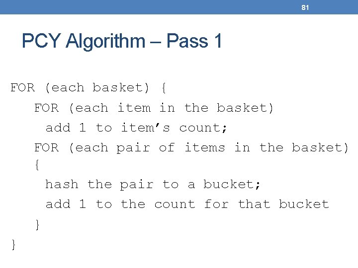
81 PCY Algorithm – Pass 1 FOR (each basket) { FOR (each item in the basket) add 1 to item’s count; FOR (each pair of items in the basket) { hash the pair to a bucket; add 1 to the count for that bucket } }

82 Observations About Buckets • A bucket is frequent if its count is at least the support threshold. • A bucket that a frequent pair hashes to is surely frequent. • We cannot use the hash table to eliminate any member of this bucket. • Even without any frequent pair, a bucket can be frequent. • Again, nothing in the bucket can be eliminated. • But in the best case, the count for a bucket is less than the support s. • Now, all pairs that hash to this bucket can be eliminated as candidates, even if the pair consists of two frequent items. • On Pass 2 (frequent pairs), we only count pairs that hash to frequent buckets.

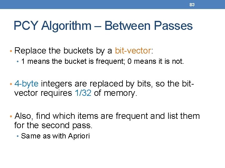
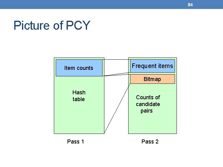
83 PCY Algorithm – Between Passes • Replace the buckets by a bit-vector: • 1 means the bucket is frequent; 0 means it is not. • 4 -byte integers are replaced by bits, so the bit- vector requires 1/32 of memory. • Also, find which items are frequent and list them for the second pass. • Same as with Apriori

84 Picture of PCY Item counts Frequent items Bitmap Hash table Pass 1 Counts of candidate pairs Pass 2

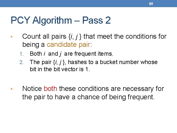
85 PCY Algorithm – Pass 2 • Count all pairs {i, j } that meet the conditions for being a candidate pair: 1. 2. • Both i and j are frequent items. The pair {i, j }, hashes to a bucket number whose bit in the bit vector is 1. Notice both these conditions are necessary for the pair to have a chance of being frequent.

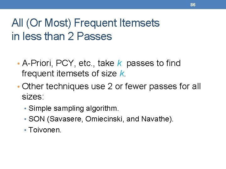
86 All (Or Most) Frequent Itemsets in less than 2 Passes • A-Priori, PCY, etc. , take k passes to find frequent itemsets of size k. • Other techniques use 2 or fewer passes for all sizes: • Simple sampling algorithm. • SON (Savasere, Omiecinski, and Navathe). • Toivonen.

87 Simple Sampling Algorithm – (1) • Take a random sample of the market baskets. • Run Apriori or one of its improvements (for sets of all sizes, not just pairs) in main memory, so you don’t pay for disk I/O each time you increase the size of itemsets. • Make sure the sample is such that there is enough space for counts.

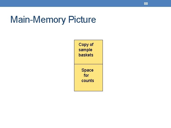
88 Main-Memory Picture Copy of sample baskets Space for counts

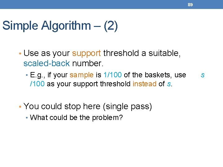
89 Simple Algorithm – (2) • Use as your support threshold a suitable, scaled-back number. • E. g. , if your sample is 1/100 of the baskets, use /100 as your support threshold instead of s. • You could stop here (single pass) • What could be the problem? s

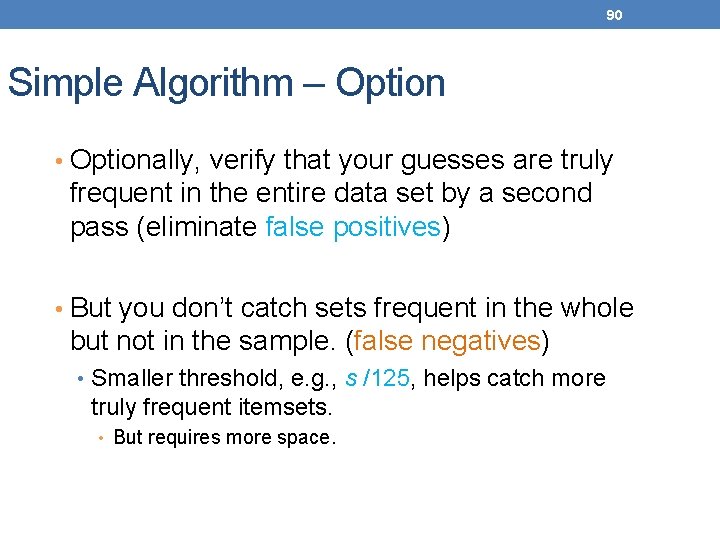
90 Simple Algorithm – Option • Optionally, verify that your guesses are truly frequent in the entire data set by a second pass (eliminate false positives) • But you don’t catch sets frequent in the whole but not in the sample. (false negatives) • Smaller threshold, e. g. , s /125, helps catch more truly frequent itemsets. • But requires more space.

91 SON Algorithm – (1) • First pass: Break the data into chunks that can be processed in main memory. • Read one chunk at the time • Find all frequent itemsets for each chunk. • Threshold = s/number of chunks • An itemset becomes a candidate if it is found to be frequent in any one or more chunks of the baskets.

92 SON Algorithm – (2) • Second pass: count all the candidate itemsets and determine which are frequent in the entire set. • Key “monotonicity” idea: an itemset cannot be frequent in the entire set of baskets unless it is frequent in at least one subset. • Why?

93 SON Algorithm – Distributed Version • This idea lends itself to distributed data mining. • If baskets are distributed among many nodes, compute frequent itemsets at each node, then distribute the candidates from each node. • Finally, accumulate the counts of all candidates.

94 Toivonen’s Algorithm – (1) • Start as in the simple sampling algorithm, but lower the threshold slightly for the sample. • Example: if the sample is 1% of the baskets, use s /125 as the support threshold rather than s /100. • Goal is to avoid missing any itemset that is frequent in the full set of baskets.

95 Toivonen’s Algorithm – (2) • Add to the itemsets that are frequent in the sample the negative border of these itemsets. • An itemset is in the negative border if it is not deemed frequent in the sample, but all its immediate subsets are.

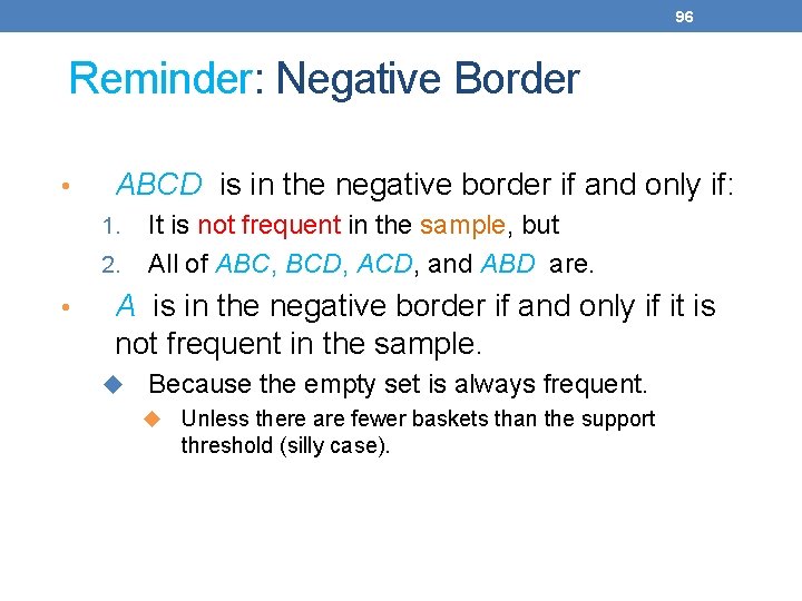
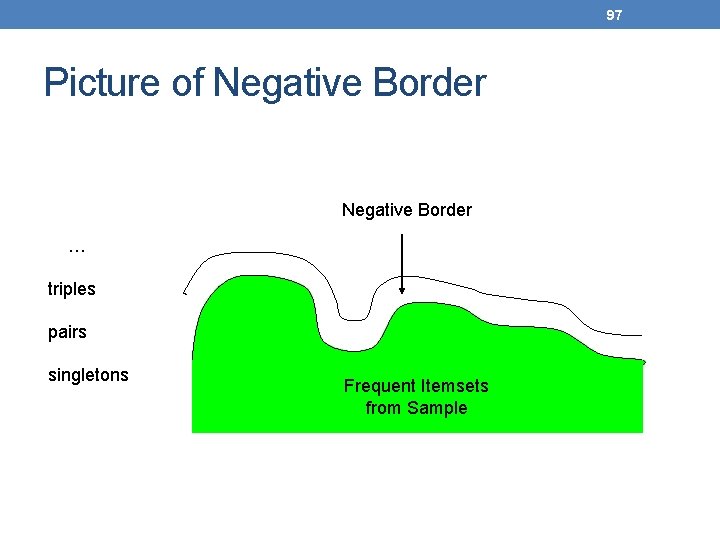
96 Reminder: Negative Border • ABCD is in the negative border if and only if: 1. 2. • It is not frequent in the sample, but All of ABC, BCD, ACD, and ABD are. A is in the negative border if and only if it is not frequent in the sample. u Because the empty set is always frequent. u Unless there are fewer baskets than the support threshold (silly case).

97 Picture of Negative Border … triples pairs singletons Frequent Itemsets from Sample

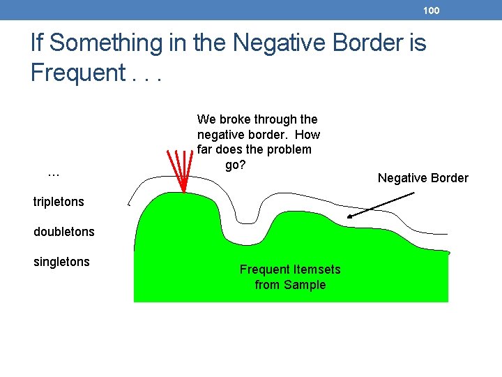
98 Toivonen’s Algorithm – (3) • In a second pass, count all candidate frequent itemsets from the first pass, and also count their negative border. • If no itemset from the negative border turns out to be frequent, then the candidates found to be frequent in the whole data are exactly the frequent itemsets.

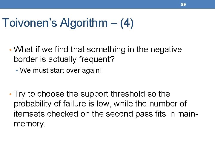
99 Toivonen’s Algorithm – (4) • What if we find that something in the negative border is actually frequent? • We must start over again! • Try to choose the support threshold so the probability of failure is low, while the number of itemsets checked on the second pass fits in mainmemory.

100 If Something in the Negative Border is Frequent. . . … We broke through the negative border. How far does the problem go? tripletons doubletons singletons Frequent Itemsets from Sample Negative Border

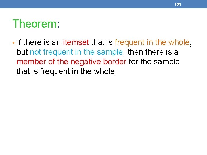
101 Theorem: • If there is an itemset that is frequent in the whole, but not frequent in the sample, then there is a member of the negative border for the sample that is frequent in the whole.

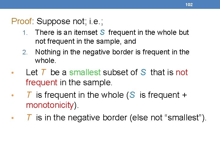
102 Proof: Suppose not; i. e. ; 1. 2. • • • There is an itemset S frequent in the whole but not frequent in the sample, and Nothing in the negative border is frequent in the whole. Let T be a smallest subset of S that is not frequent in the sample. T is frequent in the whole (S is frequent + monotonicity). T is in the negative border (else not “smallest”).

Example Border

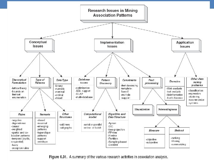
FREQUENT ITEMSET RESEARCH