What Is Association Mining l Association rule mining

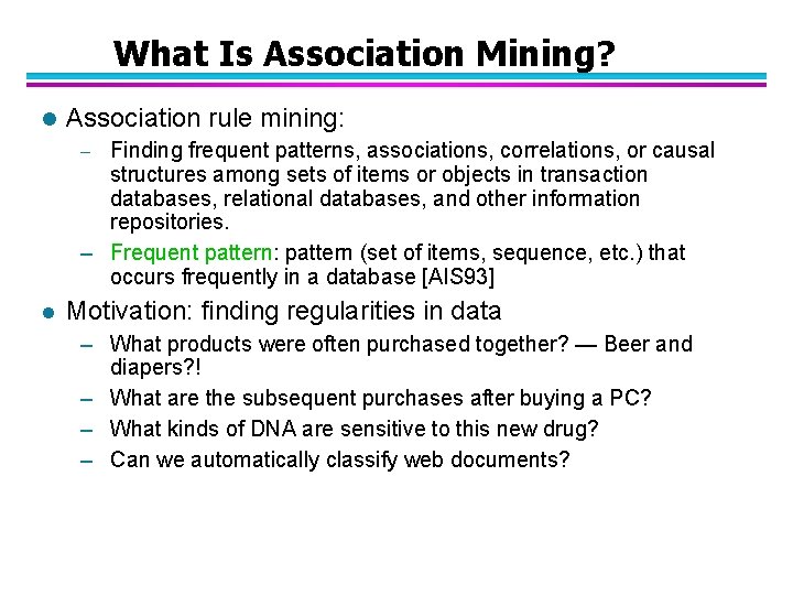
What Is Association Mining? l Association rule mining: Finding frequent patterns, associations, correlations, or causal structures among sets of items or objects in transaction databases, relational databases, and other information repositories. – Frequent pattern: pattern (set of items, sequence, etc. ) that occurs frequently in a database [AIS 93] – l Motivation: finding regularities in data – What products were often purchased together? — Beer and diapers? ! – What are the subsequent purchases after buying a PC? – What kinds of DNA are sensitive to this new drug? – Can we automatically classify web documents?

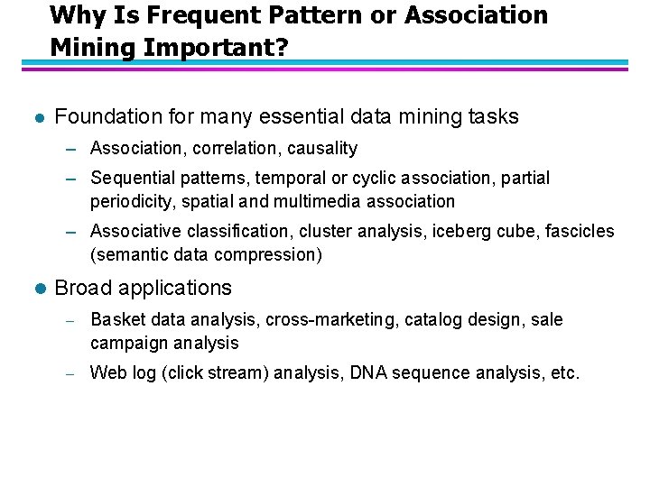
Why Is Frequent Pattern or Association Mining Important? l Foundation for many essential data mining tasks – Association, correlation, causality – Sequential patterns, temporal or cyclic association, partial periodicity, spatial and multimedia association – Associative classification, cluster analysis, iceberg cube, fascicles (semantic data compression) l Broad applications – Basket data analysis, cross-marketing, catalog design, sale campaign analysis – Web log (click stream) analysis, DNA sequence analysis, etc.

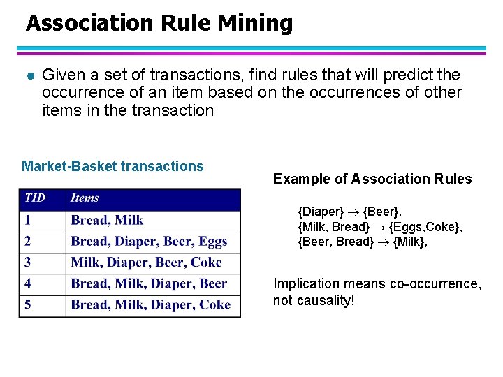
Association Rule Mining l Given a set of transactions, find rules that will predict the occurrence of an item based on the occurrences of other items in the transaction Market-Basket transactions Example of Association Rules {Diaper} {Beer}, {Milk, Bread} {Eggs, Coke}, {Beer, Bread} {Milk}, Implication means co-occurrence, not causality!

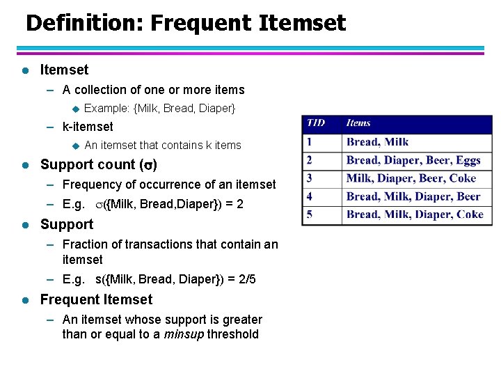
Definition: Frequent Itemset l Itemset – A collection of one or more items u Example: {Milk, Bread, Diaper} – k-itemset u l An itemset that contains k items Support count ( ) – Frequency of occurrence of an itemset – E. g. ({Milk, Bread, Diaper}) = 2 l Support – Fraction of transactions that contain an itemset – E. g. s({Milk, Bread, Diaper}) = 2/5 l Frequent Itemset – An itemset whose support is greater than or equal to a minsup threshold

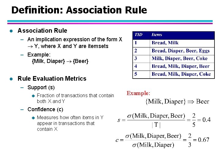
Definition: Association Rule l Association Rule – An implication expression of the form X Y, where X and Y are itemsets – Example: {Milk, Diaper} {Beer} l Rule Evaluation Metrics – Support (s) u Fraction of transactions that contain both X and Y – Confidence (c) u Measures how often items in Y appear in transactions that contain X Example:

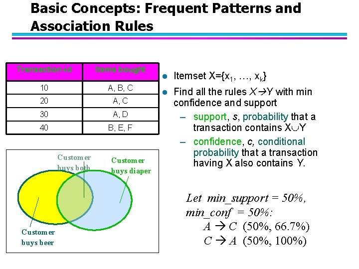
Basic Concepts: Frequent Patterns and Association Rules Transaction-id Items bought 10 A, B, C 20 A, C 30 A, D 40 B, E, F Customer buys both Customer buys beer Customer buys diaper l Itemset X={x 1, …, xk} l Find all the rules X Y with min confidence and support – support, s, probability that a transaction contains X Y – confidence, c, conditional probability that a transaction having X also contains Y. Let min_support = 50%, min_conf = 50%: A C (50%, 66. 7%) C A (50%, 100%)

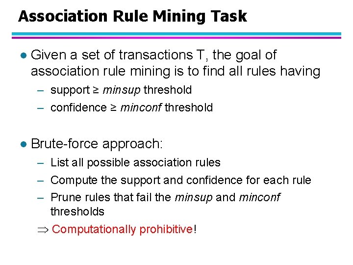
Association Rule Mining Task l Given a set of transactions T, the goal of association rule mining is to find all rules having – support ≥ minsup threshold – confidence ≥ minconf threshold l Brute-force approach: – List all possible association rules – Compute the support and confidence for each rule – Prune rules that fail the minsup and minconf thresholds Computationally prohibitive!

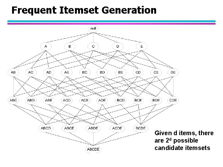
Frequent Itemset Generation Given d items, there are 2 d possible candidate itemsets

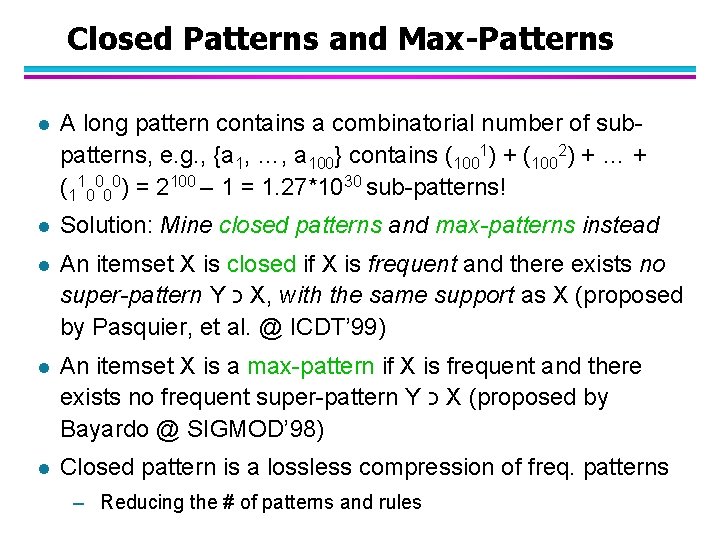
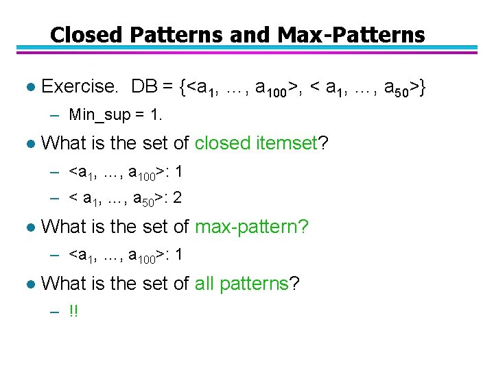
Closed Patterns and Max-Patterns l A long pattern contains a combinatorial number of subpatterns, e. g. , {a 1, …, a 100} contains (1001) + (1002) + … + (110000) = 2100 – 1 = 1. 27*1030 sub-patterns! l Solution: Mine closed patterns and max-patterns instead l An itemset X is closed if X is frequent and there exists no super-pattern Y כ X, with the same support as X (proposed by Pasquier, et al. @ ICDT’ 99) l An itemset X is a max-pattern if X is frequent and there exists no frequent super-pattern Y כ X (proposed by Bayardo @ SIGMOD’ 98) l Closed pattern is a lossless compression of freq. patterns – Reducing the # of patterns and rules

Closed Patterns and Max-Patterns l Exercise. DB = {<a 1, …, a 100>, < a 1, …, a 50>} – Min_sup = 1. l What is the set of closed itemset? – <a 1, …, a 100>: 1 – < a 1, …, a 50>: 2 l What is the set of max-pattern? – <a 1, …, a 100>: 1 l What is the set of all patterns? – !!

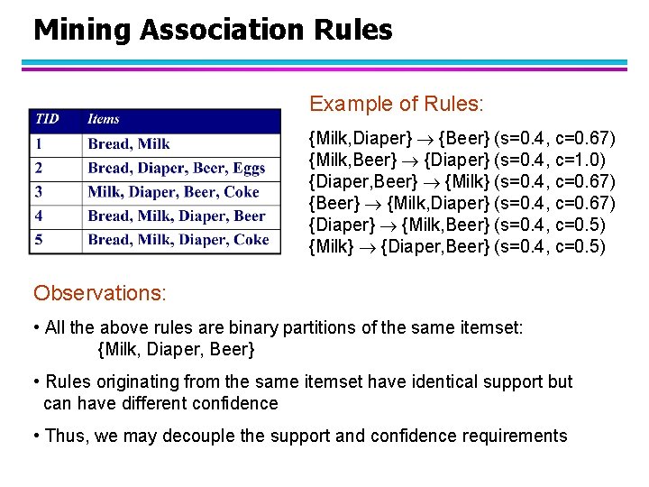
Mining Association Rules Example of Rules: {Milk, Diaper} {Beer} (s=0. 4, c=0. 67) {Milk, Beer} {Diaper} (s=0. 4, c=1. 0) {Diaper, Beer} {Milk} (s=0. 4, c=0. 67) {Beer} {Milk, Diaper} (s=0. 4, c=0. 67) {Diaper} {Milk, Beer} (s=0. 4, c=0. 5) {Milk} {Diaper, Beer} (s=0. 4, c=0. 5) Observations: • All the above rules are binary partitions of the same itemset: {Milk, Diaper, Beer} • Rules originating from the same itemset have identical support but can have different confidence • Thus, we may decouple the support and confidence requirements

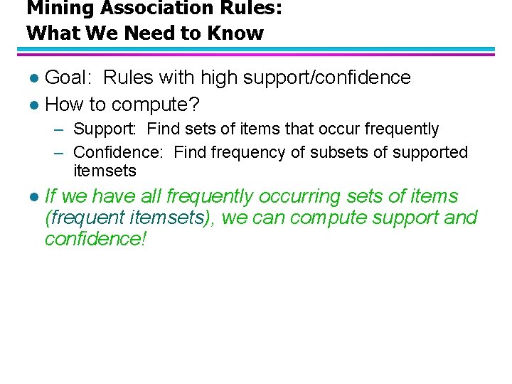
Mining Association Rules: What We Need to Know Goal: Rules with high support/confidence l How to compute? l – Support: Find sets of items that occur frequently – Confidence: Find frequency of subsets of supported itemsets l If we have all frequently occurring sets of items (frequent itemsets), we can compute support and confidence!

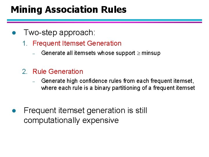
Mining Association Rules l Two-step approach: 1. Frequent Itemset Generation – Generate all itemsets whose support minsup 2. Rule Generation – l Generate high confidence rules from each frequent itemset, where each rule is a binary partitioning of a frequent itemset Frequent itemset generation is still computationally expensive

Frequent Itemset Generation Given d items, there are 2 d possible candidate itemsets

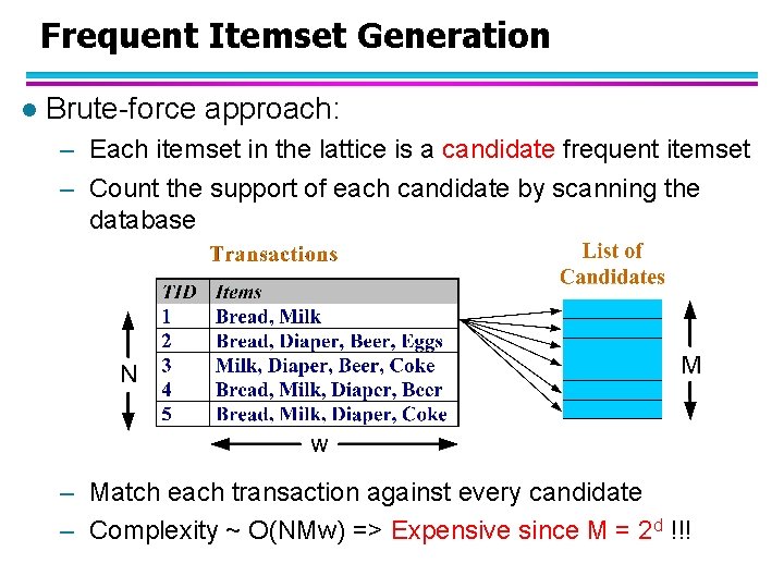
Frequent Itemset Generation l Brute-force approach: – Each itemset in the lattice is a candidate frequent itemset – Count the support of each candidate by scanning the database – Match each transaction against every candidate – Complexity ~ O(NMw) => Expensive since M = 2 d !!!

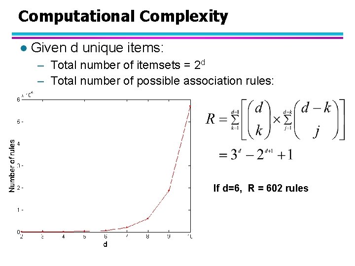
Computational Complexity l Given d unique items: – Total number of itemsets = 2 d – Total number of possible association rules: If d=6, R = 602 rules

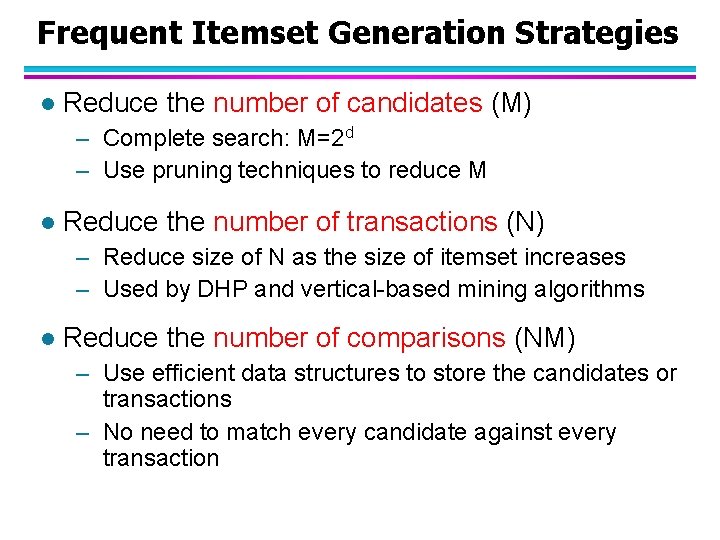
Frequent Itemset Generation Strategies l Reduce the number of candidates (M) – Complete search: M=2 d – Use pruning techniques to reduce M l Reduce the number of transactions (N) – Reduce size of N as the size of itemset increases – Used by DHP and vertical-based mining algorithms l Reduce the number of comparisons (NM) – Use efficient data structures to store the candidates or transactions – No need to match every candidate against every transaction

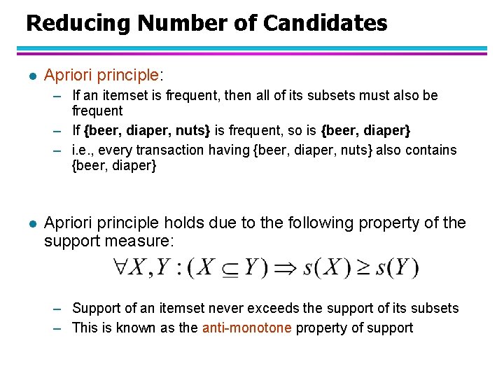
Reducing Number of Candidates l Apriori principle: – If an itemset is frequent, then all of its subsets must also be frequent – If {beer, diaper, nuts} is frequent, so is {beer, diaper} – i. e. , every transaction having {beer, diaper, nuts} also contains {beer, diaper} l Apriori principle holds due to the following property of the support measure: – Support of an itemset never exceeds the support of its subsets – This is known as the anti-monotone property of support

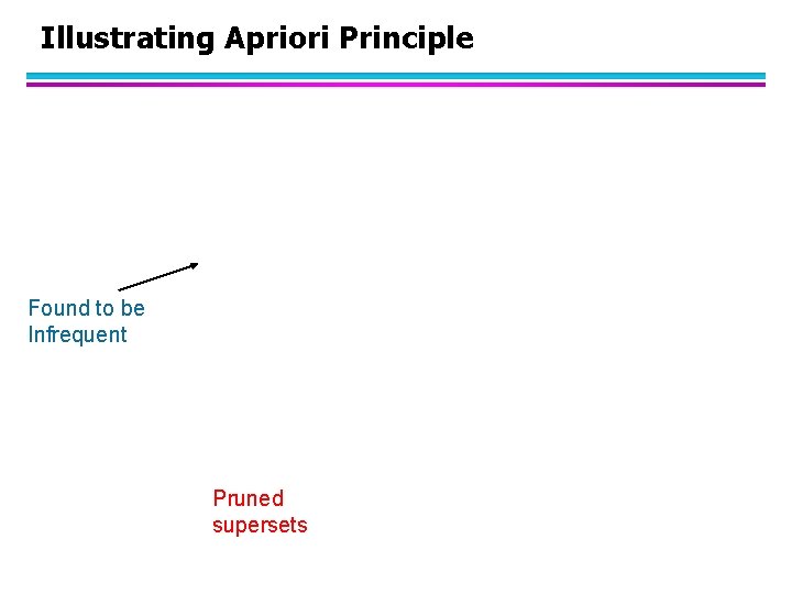
Illustrating Apriori Principle Found to be Infrequent Pruned supersets

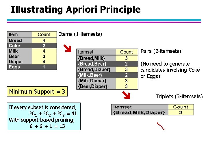
Illustrating Apriori Principle Items (1 -itemsets) Pairs (2 -itemsets) (No need to generate candidates involving Coke or Eggs) Minimum Support = 3 If every subset is considered, 6 C + 6 C = 41 1 2 3 With support-based pruning, 6 + 1 = 13 Triplets (3 -itemsets)

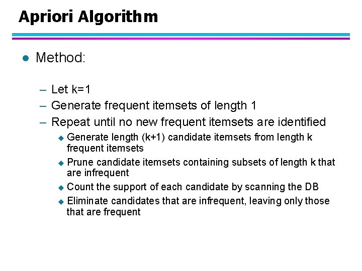
Apriori Algorithm l Method: – Let k=1 – Generate frequent itemsets of length 1 – Repeat until no new frequent itemsets are identified u Generate length (k+1) candidate itemsets from length k frequent itemsets u Prune candidate itemsets containing subsets of length k that are infrequent u Count the support of each candidate by scanning the DB u Eliminate candidates that are infrequent, leaving only those that are frequent

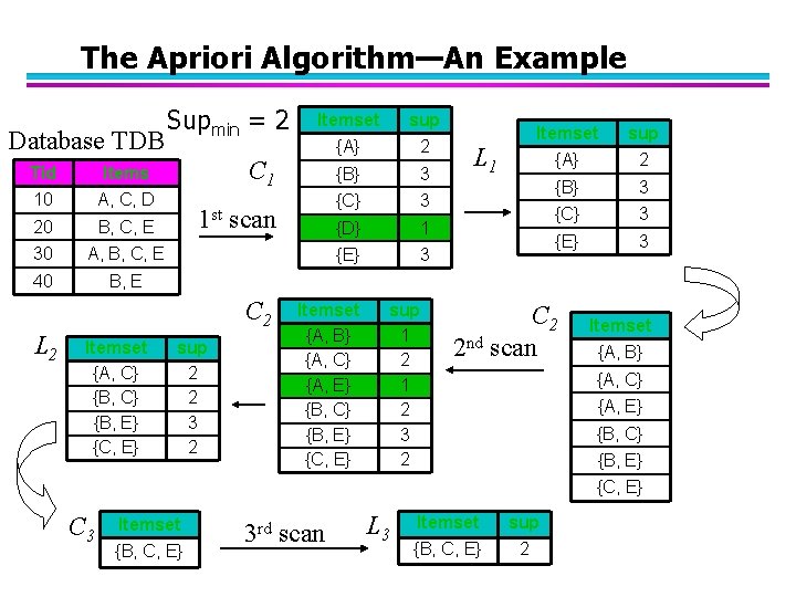
The Apriori Algorithm—An Example Database TDB Tid Items 10 A, C, D 20 B, C, E 30 A, B, C, E 40 B, E Supmin = 2 Itemset {A, C} {B, E} {C, E} sup {A} 2 {B} 3 {C} 3 {D} 1 {E} 3 C 1 1 st scan C 2 L 2 Itemset sup 2 2 3 2 Itemset {A, B} {A, C} {A, E} {B, C} {B, E} {C, E} sup 1 2 3 2 L 1 Itemset sup {A} 2 {B} 3 {C} 3 {E} 3 C 2 2 nd scan Itemset {A, B} {A, C} {A, E} {B, C} {B, E} {C, E} C 3 Itemset {B, C, E} 3 rd scan L 3 Itemset sup {B, C, E} 2

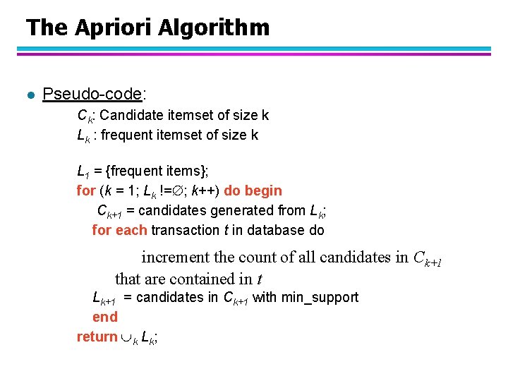
The Apriori Algorithm l Pseudo-code: Ck: Candidate itemset of size k Lk : frequent itemset of size k L 1 = {frequent items}; for (k = 1; Lk != ; k++) do begin Ck+1 = candidates generated from Lk; for each transaction t in database do increment the count of all candidates in Ck+1 that are contained in t Lk+1 = candidates in Ck+1 with min_support end return k Lk;

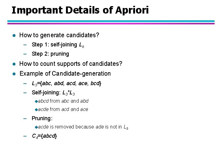
Important Details of Apriori l How to generate candidates? – Step 1: self-joining Lk – Step 2: pruning l How to count supports of candidates? l Example of Candidate-generation – L 3={abc, abd, ace, bcd} – Self-joining: L 3*L 3 uabcd from abc and abd uacde from acd and ace – Pruning: uacde is removed because ade is not in L 3 – C 4={abcd}

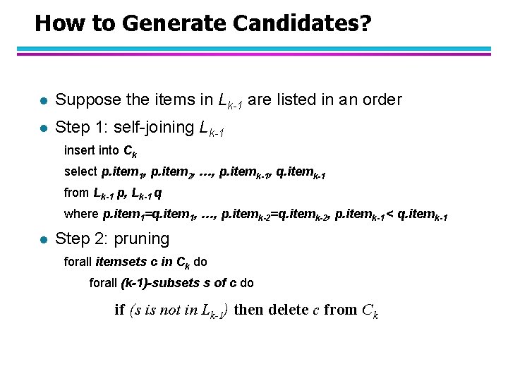
How to Generate Candidates? l Suppose the items in Lk-1 are listed in an order l Step 1: self-joining Lk-1 insert into Ck select p. item 1, p. item 2, …, p. itemk-1, q. itemk-1 from Lk-1 p, Lk-1 q where p. item 1=q. item 1, …, p. itemk-2=q. itemk-2, p. itemk-1 < q. itemk-1 l Step 2: pruning forall itemsets c in Ck do forall (k-1)-subsets s of c do if (s is not in Lk-1) then delete c from Ck

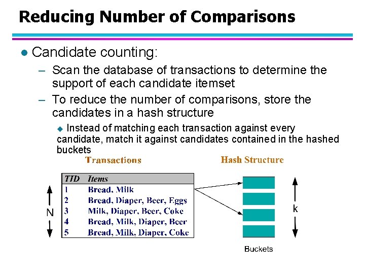
Reducing Number of Comparisons l Candidate counting: – Scan the database of transactions to determine the support of each candidate itemset – To reduce the number of comparisons, store the candidates in a hash structure Instead of matching each transaction against every candidate, match it against candidates contained in the hashed buckets u

How to Count Supports of Candidates? l Why counting supports of candidates a problem? – The total number of candidates can be very huge – l One transaction may contain many candidates Method: – Candidate itemsets are stored in a hash-tree – Leaf node of hash-tree contains a list of itemsets and counts – Interior node contains a hash table – Subset function: finds all the candidates contained in a transaction

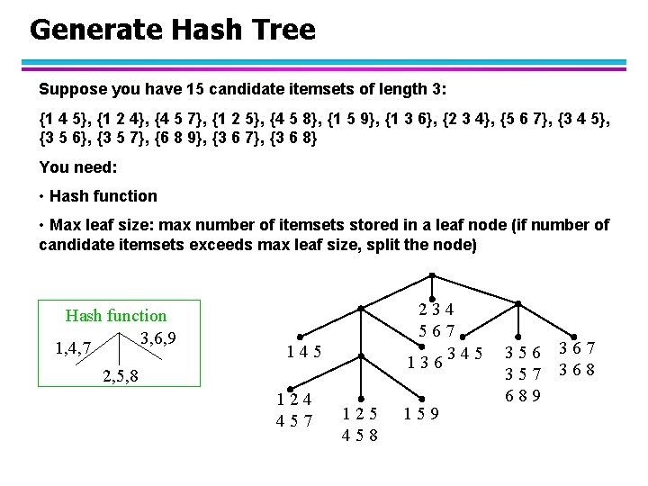
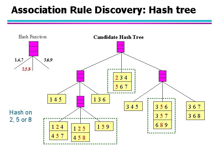
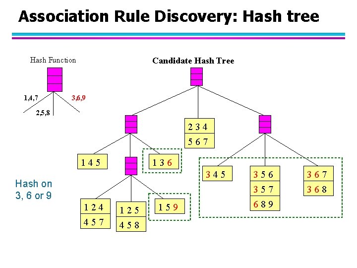
Generate Hash Tree Suppose you have 15 candidate itemsets of length 3: {1 4 5}, {1 2 4}, {4 5 7}, {1 2 5}, {4 5 8}, {1 5 9}, {1 3 6}, {2 3 4}, {5 6 7}, {3 4 5}, {3 5 6}, {3 5 7}, {6 8 9}, {3 6 7}, {3 6 8} You need: • Hash function • Max leaf size: max number of itemsets stored in a leaf node (if number of candidate itemsets exceeds max leaf size, split the node) Hash function 3, 6, 9 1, 4, 7 234 567 345 136 145 2, 5, 8 124 457 125 458 159 356 357 689 367 368

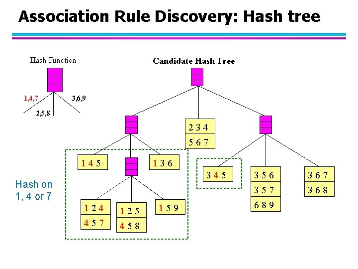
Association Rule Discovery: Hash tree Hash Function 1, 4, 7 Candidate Hash Tree 3, 6, 9 2, 5, 8 234 567 145 136 345 Hash on 1, 4 or 7 124 125 457 458 159 356 357 689 367 368

Association Rule Discovery: Hash tree Hash Function 1, 4, 7 Candidate Hash Tree 3, 6, 9 2, 5, 8 234 567 145 136 345 Hash on 2, 5 or 8 124 125 457 458 159 356 357 689 367 368

Association Rule Discovery: Hash tree Hash Function 1, 4, 7 Candidate Hash Tree 3, 6, 9 2, 5, 8 234 567 145 136 345 Hash on 3, 6 or 9 124 125 457 458 159 356 357 689 367 368

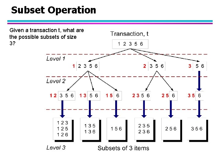
Subset Operation Given a transaction t, what are the possible subsets of size 3?

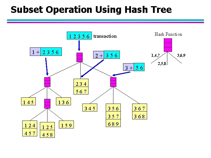
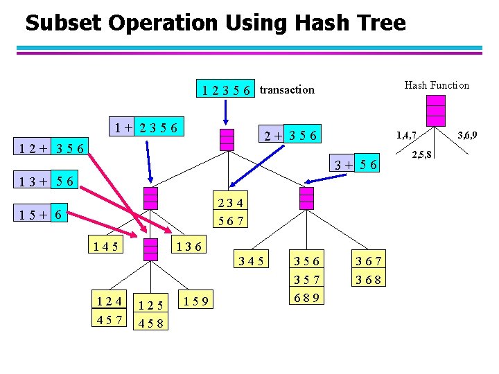
Subset Operation Using Hash Tree Hash Function 1 2 3 5 6 transaction 1+ 2356 2+ 356 1, 4, 7 3+ 56 234 567 145 136 345 124 457 125 458 159 356 357 689 367 368 2, 5, 8 3, 6, 9

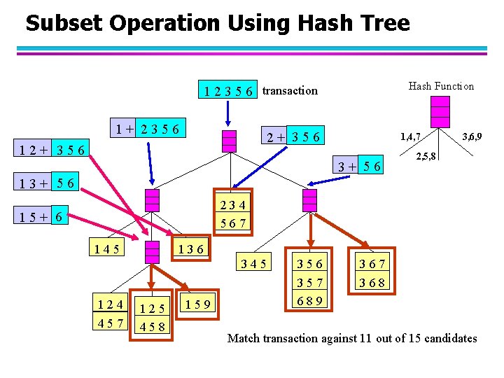
Subset Operation Using Hash Tree Hash Function 1 2 3 5 6 transaction 1+ 2356 2+ 356 1, 4, 7 3+ 56 13+ 56 234 567 15+ 6 145 136 345 124 457 125 458 159 356 357 689 367 368 2, 5, 8 3, 6, 9

Subset Operation Using Hash Tree Hash Function 1 2 3 5 6 transaction 1+ 2356 2+ 356 1, 4, 7 3+ 56 3, 6, 9 2, 5, 8 13+ 56 234 567 15+ 6 145 136 345 124 457 125 458 159 356 357 689 367 368 Match transaction against 11 out of 15 candidates

Factors Affecting Complexity l Choice of minimum support threshold – – l Dimensionality (number of items) of the data set – – l more space is needed to store support count of each item if number of frequent items also increases, both computation and I/O costs may also increase Size of database – l lowering support threshold results in more frequent itemsets this may increase number of candidates and max length of frequent itemsets since Apriori makes multiple passes, run time of algorithm may increase with number of transactions Average transaction width – transaction width increases with denser data sets – This may increase max length of frequent itemsets and traversals of hash tree (number of subsets in a transaction increases with its width)

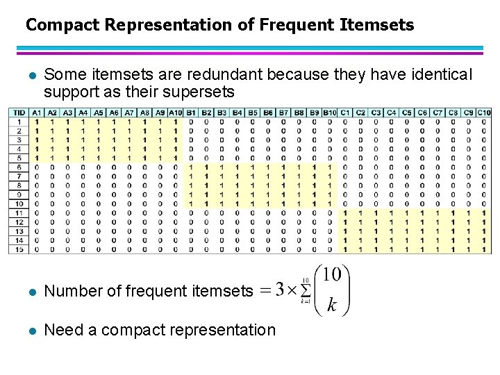
Compact Representation of Frequent Itemsets l Some itemsets are redundant because they have identical support as their supersets l Number of frequent itemsets l Need a compact representation

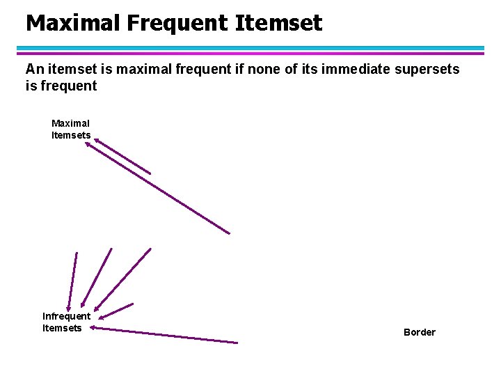
Maximal Frequent Itemset An itemset is maximal frequent if none of its immediate supersets is frequent Maximal Itemsets Infrequent Itemsets Border

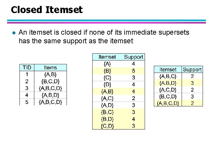
Closed Itemset l An itemset is closed if none of its immediate supersets has the same support as the itemset

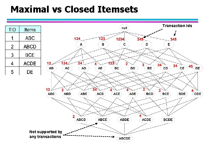
Maximal vs Closed Itemsets Transaction Ids Not supported by any transactions

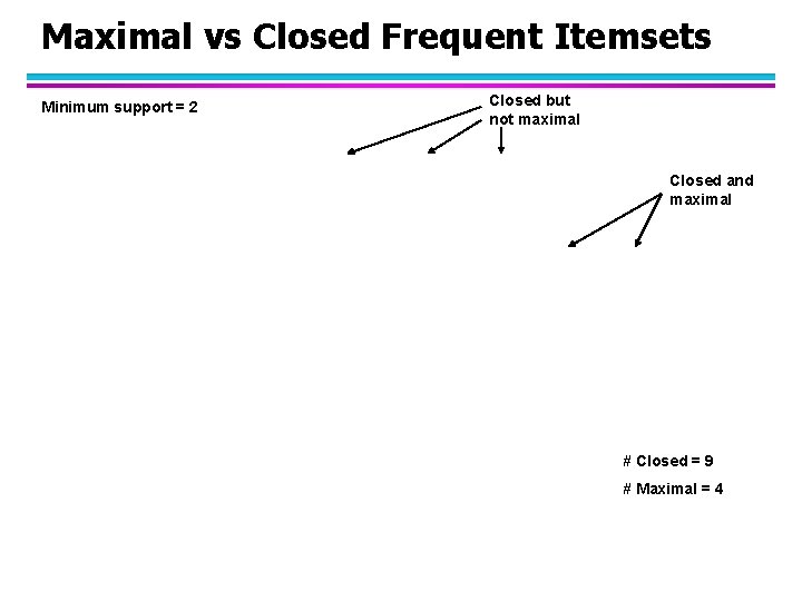
Maximal vs Closed Frequent Itemsets Minimum support = 2 Closed but not maximal Closed and maximal # Closed = 9 # Maximal = 4

Maximal vs Closed Itemsets

Alternative Methods for Frequent Itemset Generation l Traversal of Itemset Lattice – General-to-specific vs Specific-to-general

Alternative Methods for Frequent Itemset Generation l Traversal of Itemset Lattice – Equivalent Classes

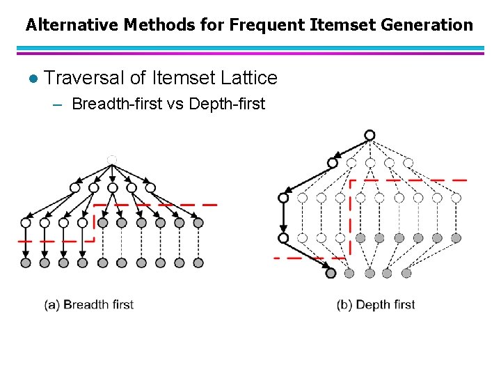
Alternative Methods for Frequent Itemset Generation l Traversal of Itemset Lattice – Breadth-first vs Depth-first

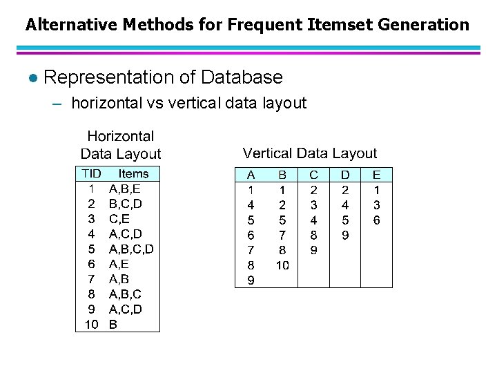
Alternative Methods for Frequent Itemset Generation l Representation of Database – horizontal vs vertical data layout

Efficient Implementation of Apriori in SQL l Hard to get good performance out of pure SQL (SQL 92) based approaches alone l Make use of object-relational extensions like UDFs, BLOBs, Table functions etc. – Get orders of magnitude improvement l S. Sarawagi, S. Thomas, and R. Agrawal. Integrating association rule mining with relational database systems: Alternatives and implications. In SIGMOD’ 98

Challenges of Frequent Pattern Mining l Challenges – Multiple scans of transaction database – Huge number of candidates – Tedious workload of support counting for candidates l Improving Apriori: general ideas – Reduce passes of transaction database scans – Shrink number of candidates – Facilitate support counting of candidates

Partition: Scan Database Only Twice l Any itemset that is potentially frequent in DB must be frequent in at least one of the partitions of DB – Scan 1: partition database and find local frequent patterns – Scan 2: consolidate global frequent patterns l A. Savasere, E. Omiecinski, and S. Navathe. An efficient algorithm for mining association in large databases. In VLDB’ 95

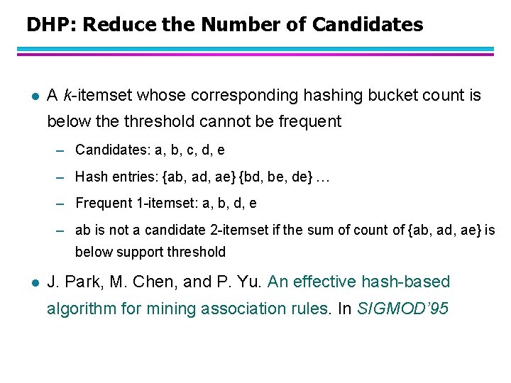
DHP: Reduce the Number of Candidates l A k-itemset whose corresponding hashing bucket count is below the threshold cannot be frequent – Candidates: a, b, c, d, e – Hash entries: {ab, ad, ae} {bd, be, de} … – Frequent 1 -itemset: a, b, d, e – ab is not a candidate 2 -itemset if the sum of count of {ab, ad, ae} is below support threshold l J. Park, M. Chen, and P. Yu. An effective hash-based algorithm for mining association rules. In SIGMOD’ 95

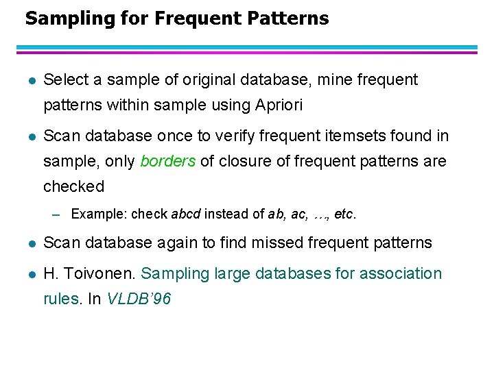
Sampling for Frequent Patterns l Select a sample of original database, mine frequent patterns within sample using Apriori l Scan database once to verify frequent itemsets found in sample, only borders of closure of frequent patterns are checked – Example: check abcd instead of ab, ac, …, etc. l Scan database again to find missed frequent patterns l H. Toivonen. Sampling large databases for association rules. In VLDB’ 96

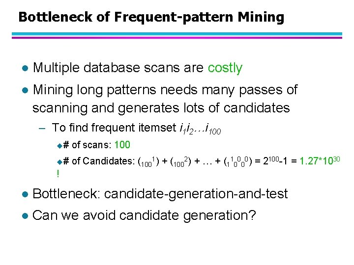
Bottleneck of Frequent-pattern Mining l Multiple database scans are costly l Mining long patterns needs many passes of scanning and generates lots of candidates – To find frequent itemset i 1 i 2…i 100 u# of scans: 100 u# of Candidates: (1001) + (1002) + … + (110000) = 2100 -1 = 1. 27*1030 ! l Bottleneck: candidate-generation-and-test l Can we avoid candidate generation?

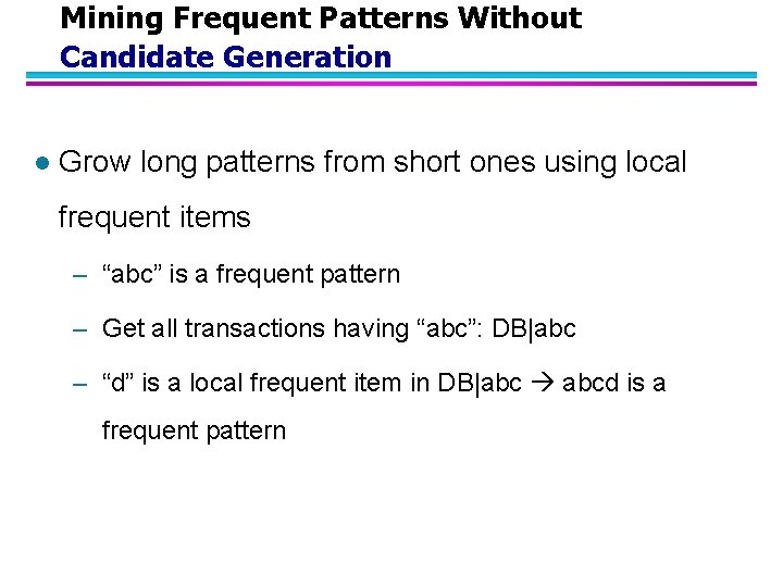
Mining Frequent Patterns Without Candidate Generation l Grow long patterns from short ones using local frequent items – “abc” is a frequent pattern – Get all transactions having “abc”: DB|abc – “d” is a local frequent item in DB|abc abcd is a frequent pattern

FP-growth Algorithm l Use a compressed representation of the database using an FP-tree l Once an FP-tree has been constructed, it uses a recursive divide-and-conquer approach to mine the frequent itemsets

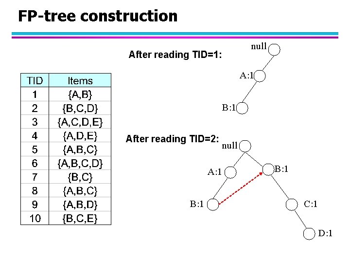
FP-tree construction null After reading TID=1: A: 1 B: 1 After reading TID=2: A: 1 B: 1 null B: 1 C: 1 D: 1

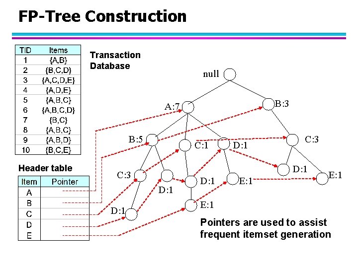
FP-Tree Construction Transaction Database null B: 3 A: 7 B: 5 Header table C: 1 C: 3 D: 1 D: 1 E: 1 Pointers are used to assist frequent itemset generation

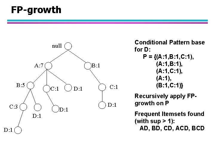
FP-growth C: 1 Conditional Pattern base for D: P = {(A: 1, B: 1, C: 1), (A: 1, B: 1), (A: 1, C: 1), (A: 1), (B: 1, C: 1)} D: 1 Recursively apply FPgrowth on P null A: 7 B: 5 C: 1 C: 3 D: 1 B: 1 D: 1 Frequent Itemsets found (with sup > 1): AD, BD, CD, ACD, BCD

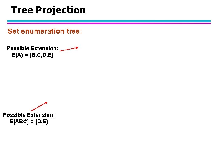
Tree Projection Set enumeration tree: Possible Extension: E(A) = {B, C, D, E} Possible Extension: E(ABC) = {D, E}

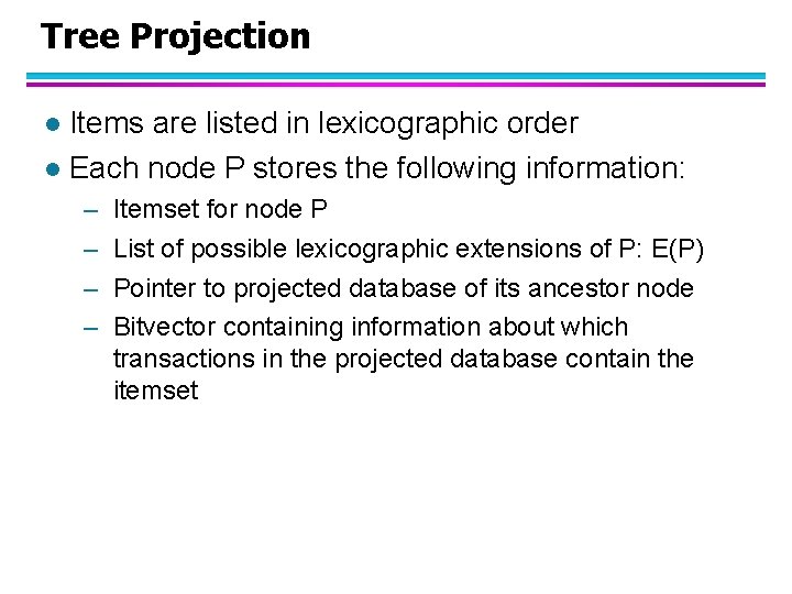
Tree Projection Items are listed in lexicographic order l Each node P stores the following information: l – – Itemset for node P List of possible lexicographic extensions of P: E(P) Pointer to projected database of its ancestor node Bitvector containing information about which transactions in the projected database contain the itemset

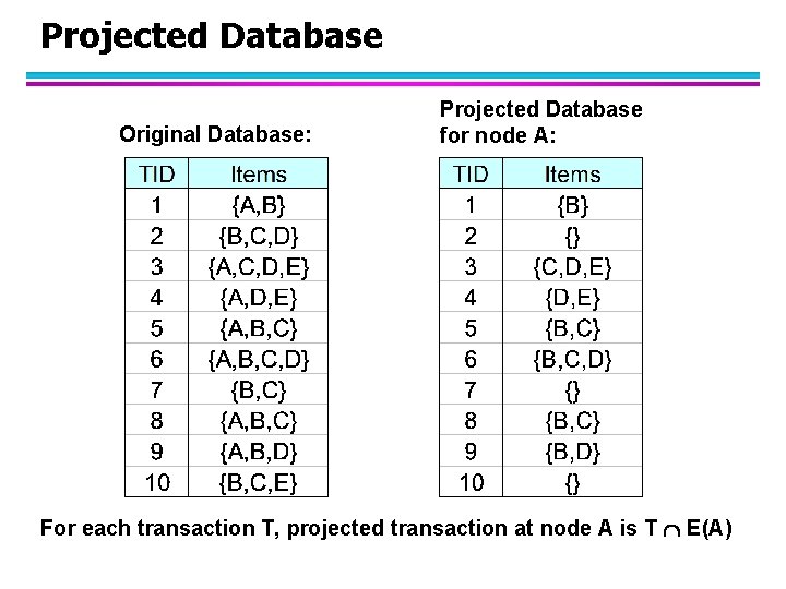
Projected Database Original Database: Projected Database for node A: For each transaction T, projected transaction at node A is T E(A)

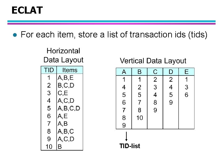
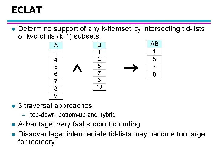
ECLAT l For each item, store a list of transaction ids (tids) TID-list

ECLAT l Determine support of any k-itemset by intersecting tid-lists of two of its (k-1) subsets. l 3 traversal approaches: – top-down, bottom-up and hybrid l l Advantage: very fast support counting Disadvantage: intermediate tid-lists may become too large for memory

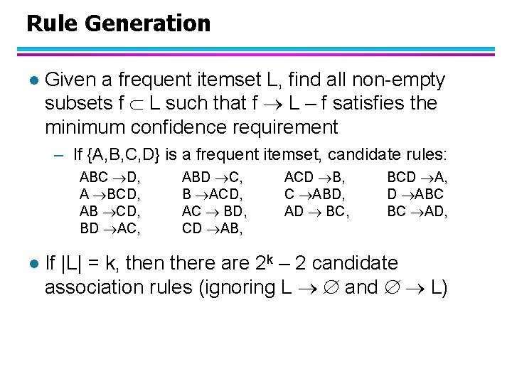
Rule Generation l Given a frequent itemset L, find all non-empty subsets f L such that f L – f satisfies the minimum confidence requirement – If {A, B, C, D} is a frequent itemset, candidate rules: ABC D, A BCD, AB CD, BD AC, l ABD C, B ACD, AC BD, CD AB, ACD B, C ABD, AD BC, BCD A, D ABC BC AD, If |L| = k, then there are 2 k – 2 candidate association rules (ignoring L and L)

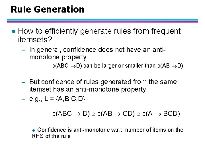
Rule Generation l How to efficiently generate rules from frequent itemsets? – In general, confidence does not have an antimonotone property c(ABC D) can be larger or smaller than c(AB D) – But confidence of rules generated from the same itemset has an anti-monotone property – e. g. , L = {A, B, C, D}: c(ABC D) c(AB CD) c(A BCD) Confidence is anti-monotone w. r. t. number of items on the RHS of the rule u

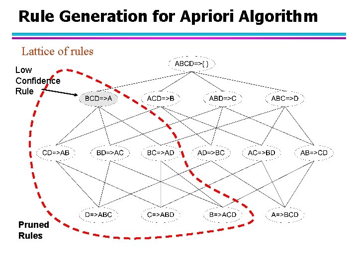
Rule Generation for Apriori Algorithm Lattice of rules Low Confidence Rule Pruned Rules

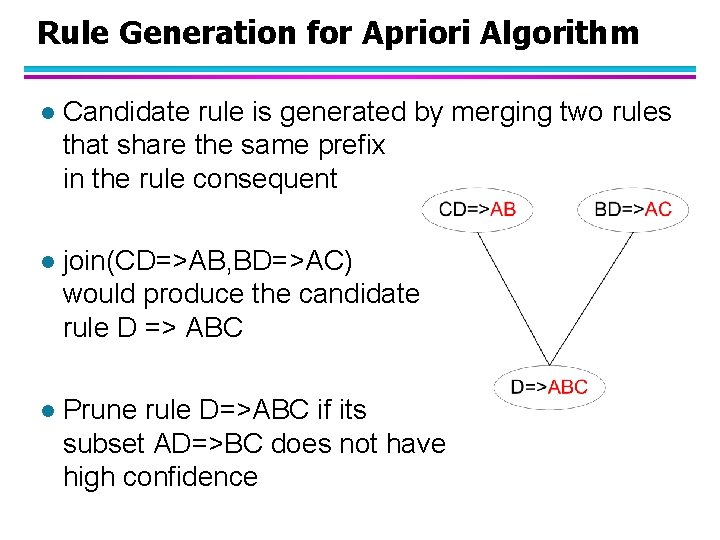
Rule Generation for Apriori Algorithm l Candidate rule is generated by merging two rules that share the same prefix in the rule consequent l join(CD=>AB, BD=>AC) would produce the candidate rule D => ABC l Prune rule D=>ABC if its subset AD=>BC does not have high confidence

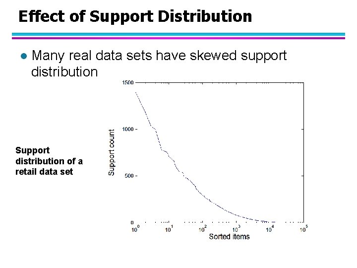
Effect of Support Distribution l Many real data sets have skewed support distribution Support distribution of a retail data set