DATA MINING LECTURE 3 Frequent Itemsets Association Rules

DATA MINING LECTURE 3 Frequent Itemsets Association Rules

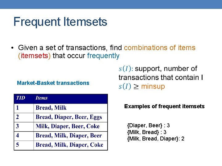
Frequent Itemsets • Given a set of transactions, find combinations of items (itemsets) that occur frequently Market-Basket transactions Examples of frequent itemsets {Diaper, Beer} : 3 {Milk, Bread, Diaper}: 2

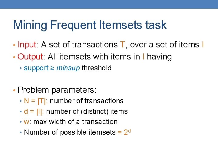
Mining Frequent Itemsets task • Input: A set of transactions T, over a set of items I • Output: All itemsets with items in I having • support ≥ minsup threshold • Problem parameters: • N = |T|: number of transactions • d = |I|: number of (distinct) items • w: max width of a transaction • Number of possible itemsets = 2 d

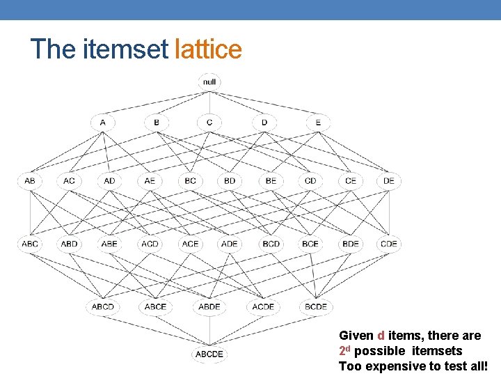
The itemset lattice Given d items, there are 2 d possible itemsets Too expensive to test all!

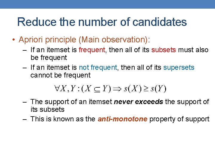
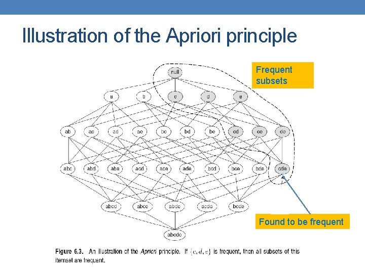
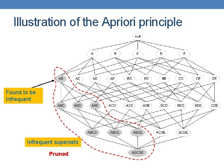
Reduce the number of candidates • Apriori principle (Main observation): – If an itemset is frequent, then all of its subsets must also be frequent – If an itemset is not frequent, then all of its supersets cannot be frequent – The support of an itemset never exceeds the support of its subsets – This is known as the anti-monotone property of support

Illustration of the Apriori principle Frequent subsets Found to be frequent

Illustration of the Apriori principle Found to be Infrequent supersets Pruned

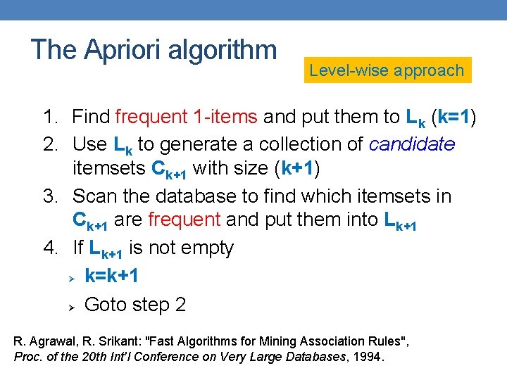
The Apriori algorithm Level-wise approach 1. Find frequent 1 -items and put them to Lk (k=1) 2. Use Lk to generate a collection of candidate itemsets Ck+1 with size (k+1) 3. Scan the database to find which itemsets in Ck+1 are frequent and put them into Lk+1 4. If Lk+1 is not empty k=k+1 Goto step 2 R. Agrawal, R. Srikant: "Fast Algorithms for Mining Association Rules", Proc. of the 20 th Int'l Conference on Very Large Databases, 1994.

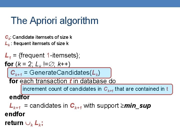
The Apriori algorithm Ck: Candidate itemsets of size k Lk : frequent itemsets of size k L 1 = {frequent 1 -itemsets}; for (k = 2; Lk != ; k++) Ck+1 = Generate. Candidates(Lk) for each transaction t in database do increment count of candidates in Ck+1 that are contained in t endfor Lk+1 = candidates in Ck+1 with support ≥min_sup endfor return k Lk;

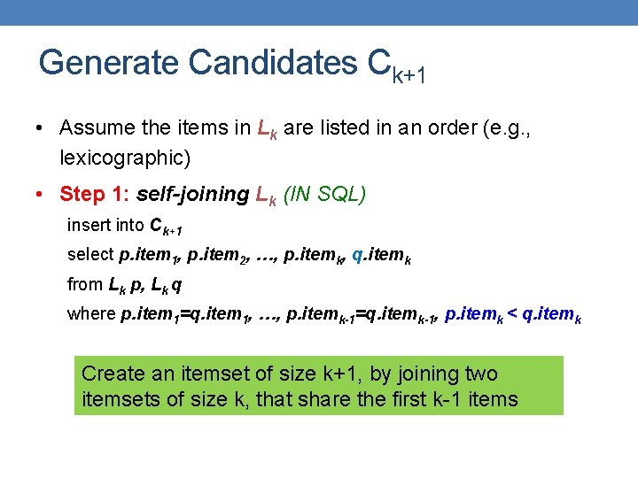
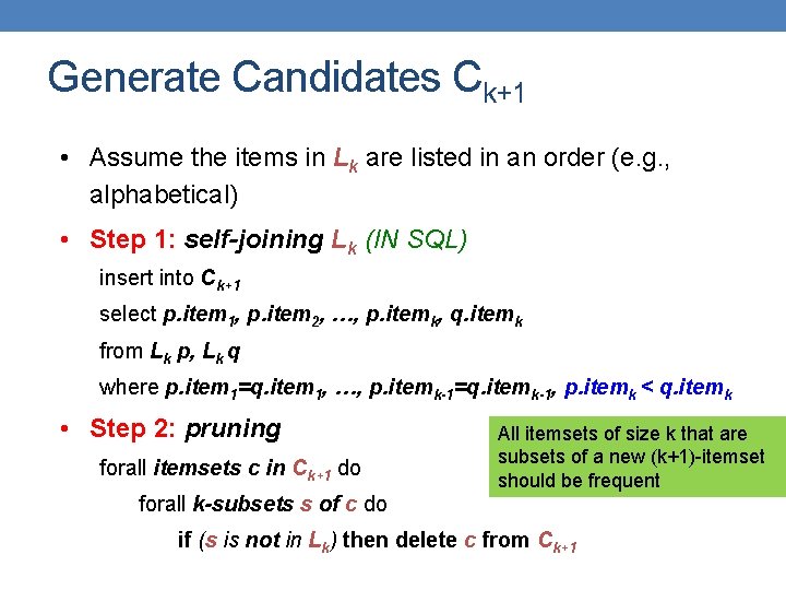
Generate Candidates Ck+1 • Assume the items in Lk are listed in an order (e. g. , lexicographic) • Step 1: self-joining Lk (IN SQL) insert into Ck+1 select p. item 1, p. item 2, …, p. itemk, q. itemk from Lk p, Lk q where p. item 1=q. item 1, …, p. itemk-1=q. itemk-1, p. itemk < q. itemk Create an itemset of size k+1, by joining two itemsets of size k, that share the first k-1 items

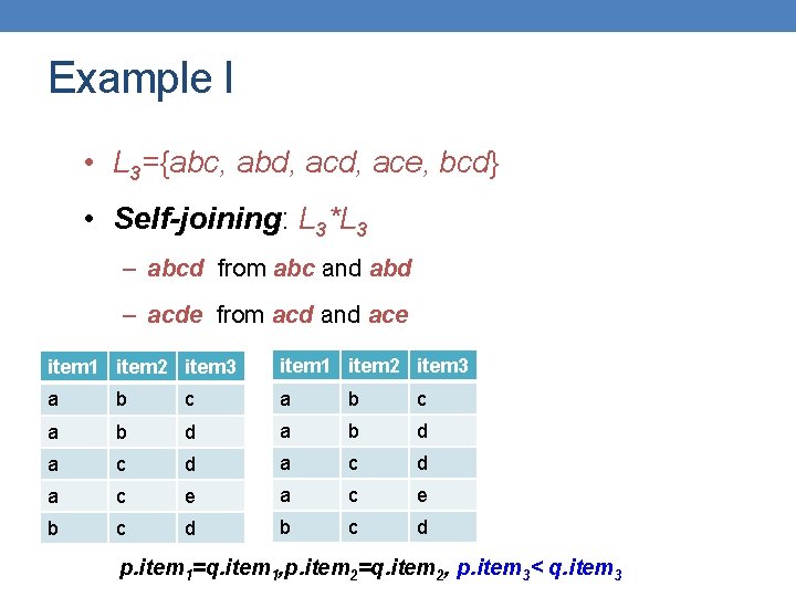
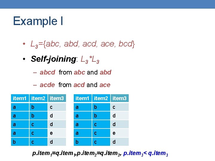
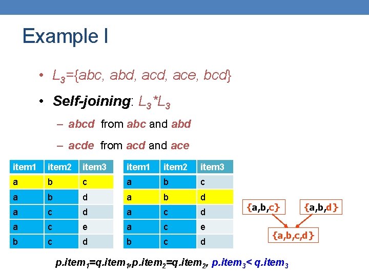
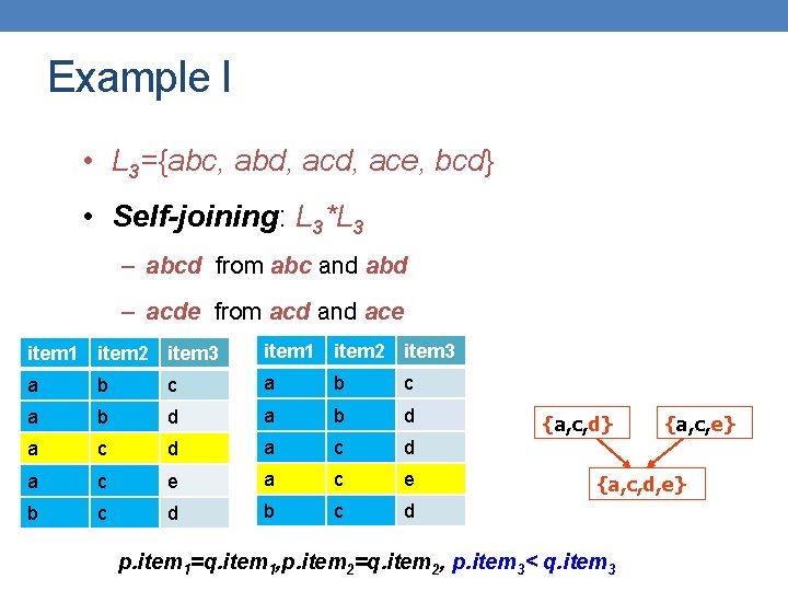
Example I • L 3={abc, abd, ace, bcd} • Self-joining: L 3*L 3 – abcd from abc and abd – acde from acd and ace item 1 item 2 item 3 a b c a b d a c e b c d p. item 1=q. item 1, p. item 2=q. item 2, p. item 3< q. item 3

Example I • L 3={abc, abd, ace, bcd} • Self-joining: L 3*L 3 – abcd from abc and abd – acde from acd and ace item 1 item 2 item 3 a b c a b d a c e b c d p. item 1=q. item 1, p. item 2=q. item 2, p. item 3< q. item 3

Example I • L 3={abc, abd, ace, bcd} • Self-joining: L 3*L 3 – abcd from abc and abd – acde from acd and ace item 1 item 2 item 3 a b c a b d a c e b c d {a, b, c} {a, b, d} {a, b, c, d} p. item 1=q. item 1, p. item 2=q. item 2, p. item 3< q. item 3

Example I • L 3={abc, abd, ace, bcd} • Self-joining: L 3*L 3 – abcd from abc and abd – acde from acd and ace item 1 item 2 item 3 a b c a b d a c e b c d {a, c, d} {a, c, e} {a, c, d, e} p. item 1=q. item 1, p. item 2=q. item 2, p. item 3< q. item 3

Generate Candidates Ck+1 • Assume the items in Lk are listed in an order (e. g. , alphabetical) • Step 1: self-joining Lk (IN SQL) insert into Ck+1 select p. item 1, p. item 2, …, p. itemk, q. itemk from Lk p, Lk q where p. item 1=q. item 1, …, p. itemk-1=q. itemk-1, p. itemk < q. itemk • Step 2: pruning forall itemsets c in Ck+1 do All itemsets of size k that are subsets of a new (k+1)-itemset should be frequent forall k-subsets s of c do if (s is not in Lk) then delete c from Ck+1

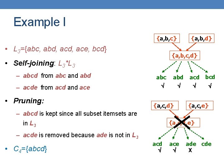
Example I {a, b, c} • L 3={abc, abd, ace, bcd} {a, b, c, d} • Self-joining: L 3*L 3 – abcd from abc and abc abd acd bcd – acde from acd and ace • Pruning: {a, c, d} {a, c, e} – abcd is kept since all subset itemsets are {a, c, d, e} in L 3 – acde is removed because ade is not in L 3 • C 4={abcd} acd ace ade cde X

The Apriori algorithm Ck: Candidate itemsets of size k Lk : frequent itemsets of size k L 1 = {frequent 1 -itemsets}; for (k = 2; Lk != ; k++) Ck+1 = Generate. Candidates(Lk) for each transaction t in database do increment count of candidates in Ck+1 that are contained in t endfor Lk+1 = candidates in Ck+1 with support ≥min_sup endfor return k Lk;

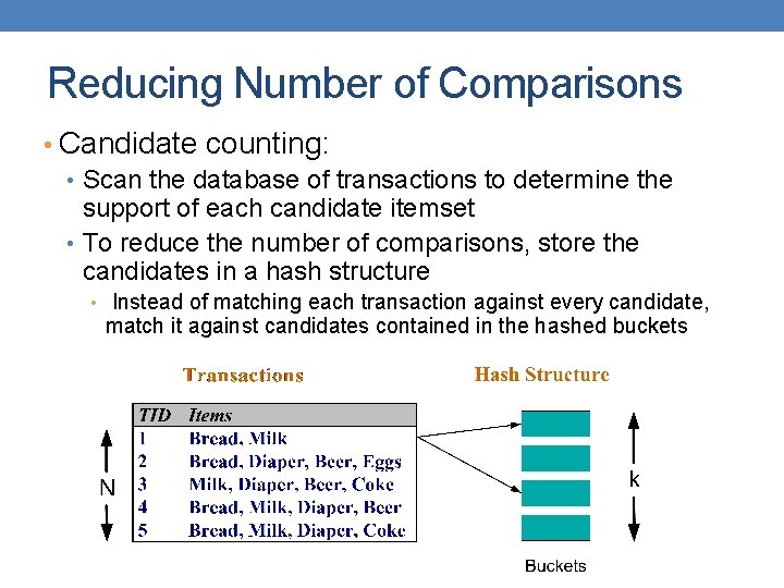
Reducing Number of Comparisons • Candidate counting: • Scan the database of transactions to determine the support of each candidate itemset • To reduce the number of comparisons, store the candidates in a hash structure • Instead of matching each transaction against every candidate, match it against candidates contained in the hashed buckets

ASSOCIATION RULES

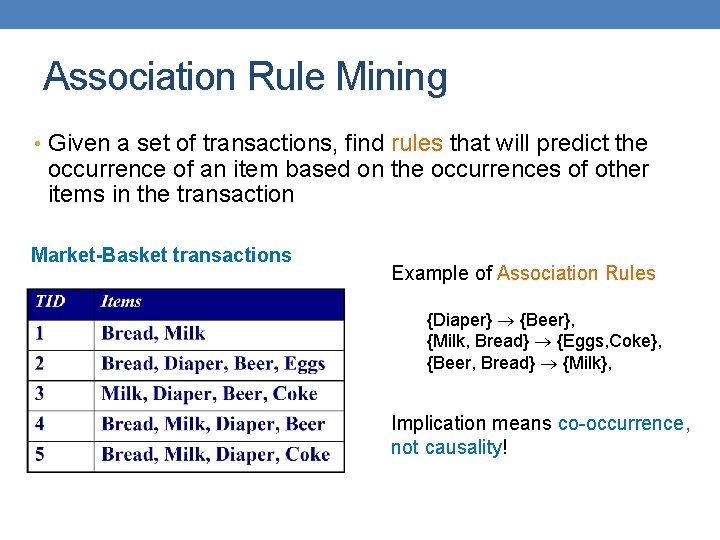
Association Rule Mining • Given a set of transactions, find rules that will predict the occurrence of an item based on the occurrences of other items in the transaction Market-Basket transactions Example of Association Rules {Diaper} {Beer}, {Milk, Bread} {Eggs, Coke}, {Beer, Bread} {Milk}, Implication means co-occurrence, not causality!

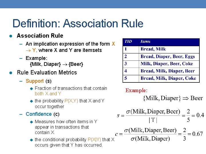
Definition: Association Rule l Association Rule – An implication expression of the form X Y, where X and Y are itemsets – Example: {Milk, Diaper} {Beer} l Rule Evaluation Metrics – Support (s) u Fraction of transactions that contain both X and Y u the probability P(X, Y) that X and Y occur together – Confidence (c) u Measures how often items in Y appear in transactions that contain X u the conditional probability P(X|Y) that X occurs given that Y has occurred. Example:

Association Rule Mining Task • Input: A set of transactions T, over a set of items I • Output: All rules with items in I having • support ≥ minsup threshold • confidence ≥ minconf threshold

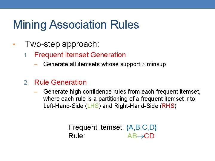
Mining Association Rules • Two-step approach: 1. Frequent Itemset Generation – Generate all itemsets whose support minsup 2. Rule Generation – Generate high confidence rules from each frequent itemset, where each rule is a partitioning of a frequent itemset into Left-Hand-Side (LHS) and Right-Hand-Side (RHS) Frequent itemset: {A, B, C, D} Rule: AB CD

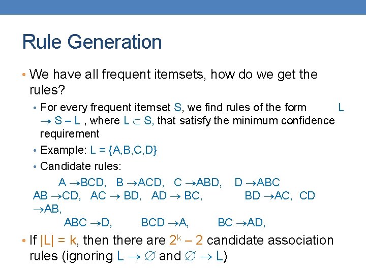
Rule Generation • We have all frequent itemsets, how do we get the rules? • For every frequent itemset S, we find rules of the form S – L , where L S, that satisfy the minimum confidence requirement • Example: L = {A, B, C, D} • Candidate rules: A BCD, B ACD, C ABD, D ABC AB CD, AC BD, AD BC, BD AC, CD AB, ABC D, BCD A, BC AD, • If |L| = k, then there are 2 k – 2 candidate association rules (ignoring L and L) L

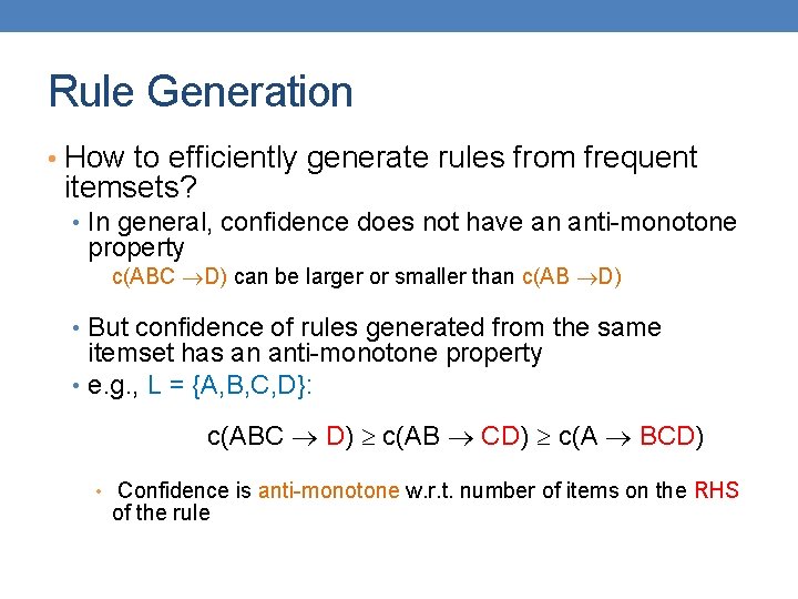
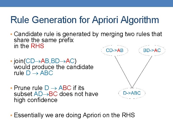
Rule Generation • How to efficiently generate rules from frequent itemsets? • In general, confidence does not have an anti-monotone property c(ABC D) can be larger or smaller than c(AB D) • But confidence of rules generated from the same itemset has an anti-monotone property • e. g. , L = {A, B, C, D}: c(ABC D) c(AB CD) c(A BCD) • Confidence is anti-monotone w. r. t. number of items on the RHS of the rule

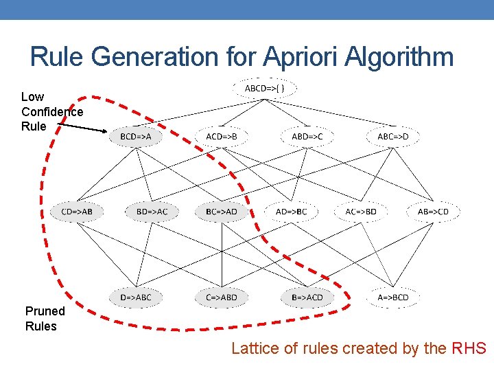
Rule Generation for Apriori Algorithm Low Confidence Rule Pruned Rules Lattice of rules created by the RHS

Rule Generation for Apriori Algorithm • Candidate rule is generated by merging two rules that share the same prefix in the RHS • join(CD AB, BD AC) would produce the candidate rule D ABC • Prune rule D ABC if its subset AD BC does not have high confidence • Essentially we are doing Apriori on the RHS

RESULT POST-PROCESSING

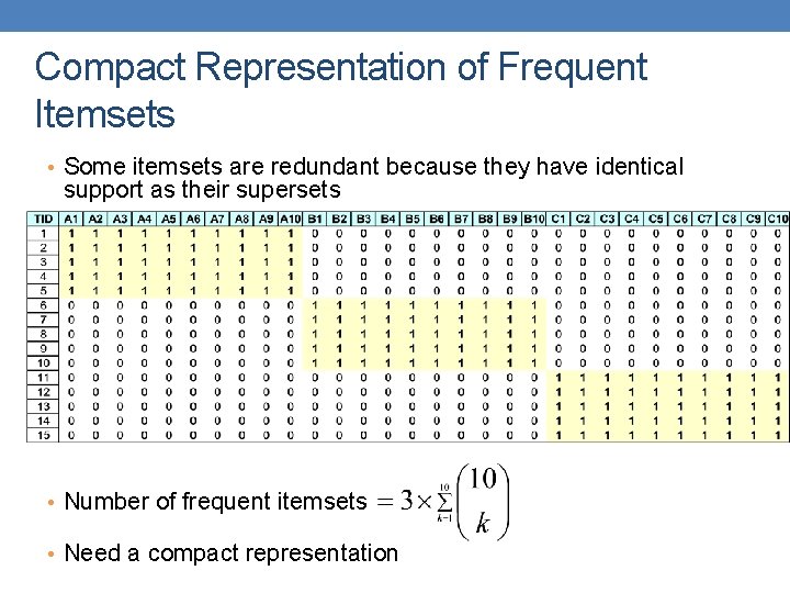
Compact Representation of Frequent Itemsets • Some itemsets are redundant because they have identical support as their supersets • Number of frequent itemsets • Need a compact representation

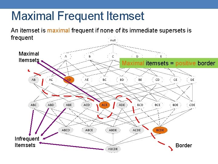
Maximal Frequent Itemset An itemset is maximal frequent if none of its immediate supersets is frequent Maximal Itemsets Infrequent Itemsets Maximal itemsets = positive border Border

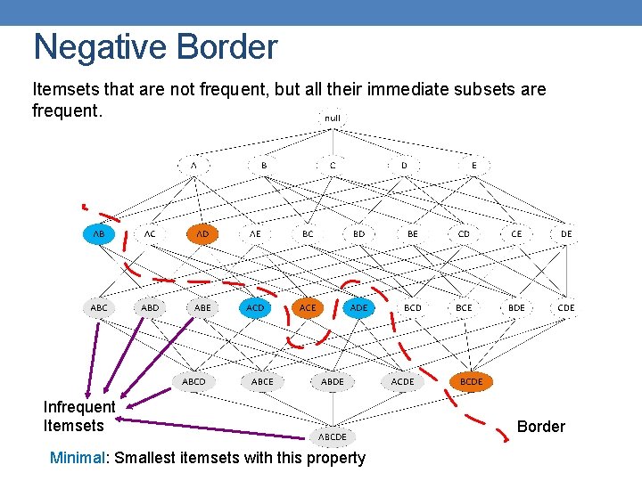
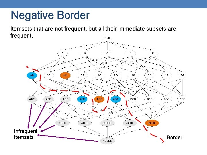
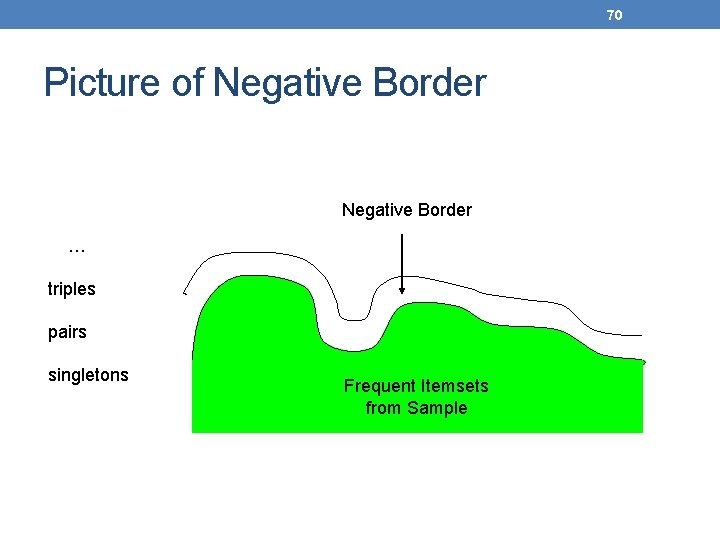
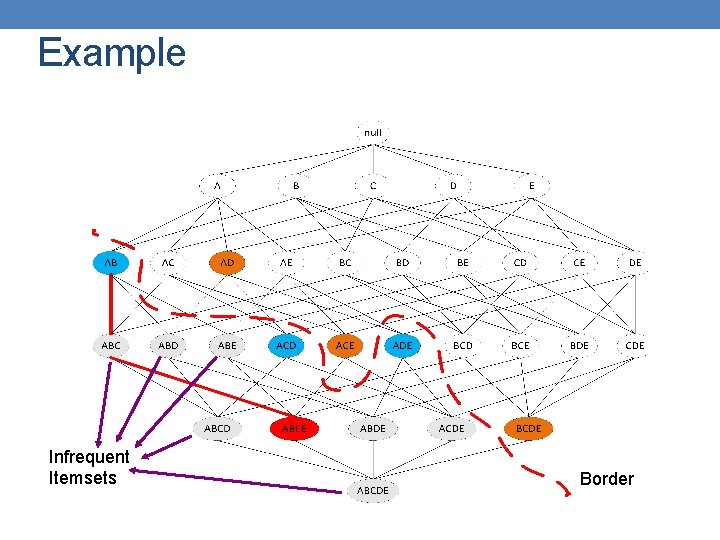
Negative Border Itemsets that are not frequent, but all their immediate subsets are frequent. Infrequent Itemsets Minimal: Smallest itemsets with this property Border

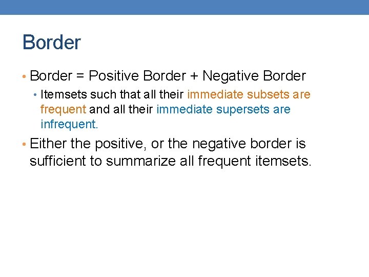
Border • Border = Positive Border + Negative Border • Itemsets such that all their immediate subsets are frequent and all their immediate supersets are infrequent. • Either the positive, or the negative border is sufficient to summarize all frequent itemsets.

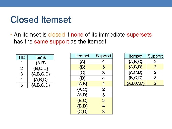
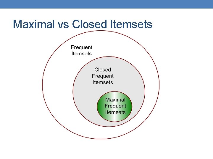
Closed Itemset • An itemset is closed if none of its immediate supersets has the same support as the itemset

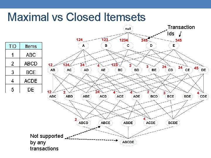
Maximal vs Closed Itemsets Transaction Ids Not supported by any transactions

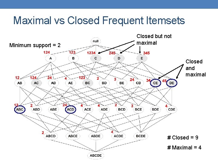
Maximal vs Closed Frequent Itemsets Minimum support = 2 Closed but not maximal Closed and maximal # Closed = 9 # Maximal = 4

Maximal vs Closed Itemsets

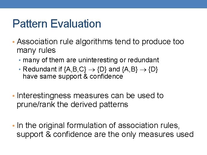
Pattern Evaluation • Association rule algorithms tend to produce too many rules • many of them are uninteresting or redundant • Redundant if {A, B, C} {D} and {A, B} {D} have same support & confidence • Interestingness measures can be used to prune/rank the derived patterns • In the original formulation of association rules, support & confidence are the only measures used

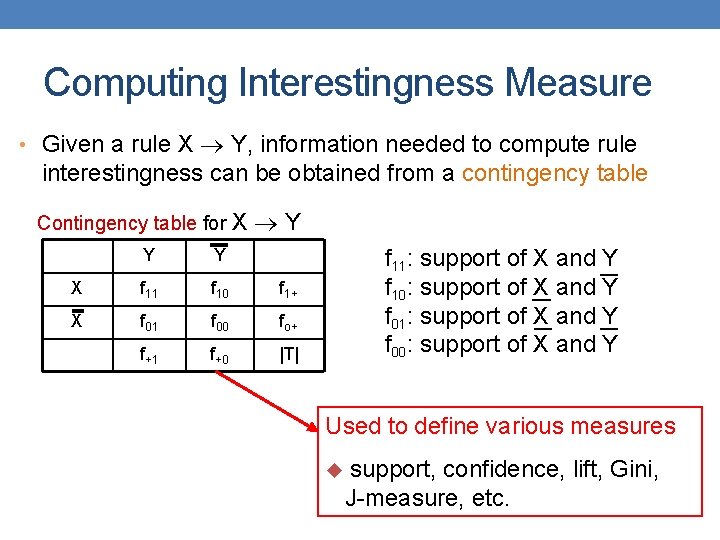
Computing Interestingness Measure • Given a rule X Y, information needed to compute rule interestingness can be obtained from a contingency table Contingency table for X Y Y Y X f 11 f 10 f 1+ X f 01 f 00 fo+ f+1 f+0 |T| f 11: support of X and Y f 10: support of X and Y f 01: support of X and Y f 00: support of X and Y Used to define various measures u support, confidence, lift, Gini, J-measure, etc.

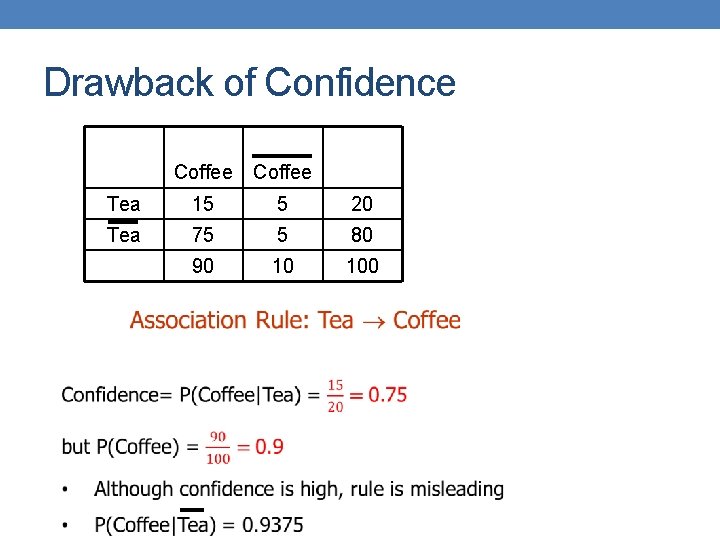
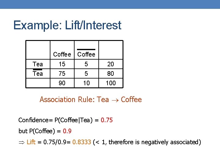
Drawback of Confidence Coffee Tea 15 5 20 Tea 75 5 80 90 10 100

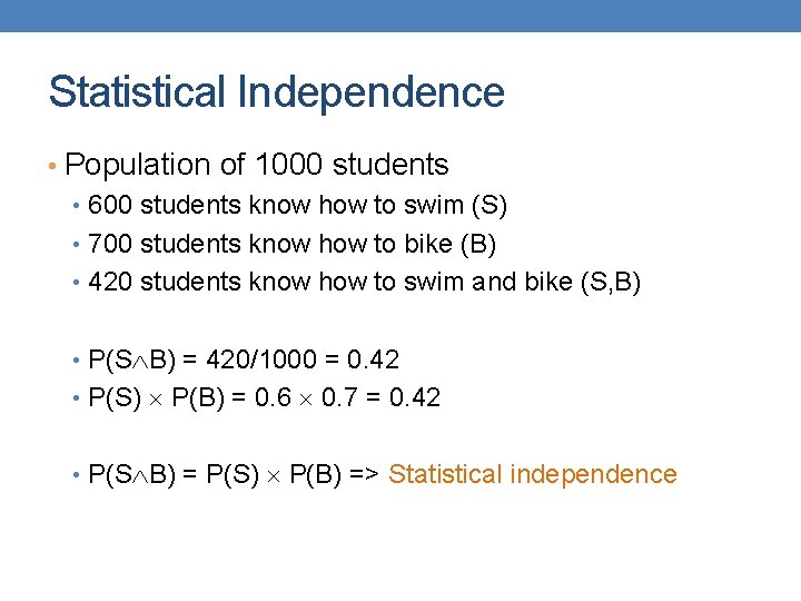
Statistical Independence • Population of 1000 students • 600 students know how to swim (S) • 700 students know how to bike (B) • 420 students know how to swim and bike (S, B) • P(S B) = 420/1000 = 0. 42 • P(S) P(B) = 0. 6 0. 7 = 0. 42 • P(S B) = P(S) P(B) => Statistical independence

Statistical Independence • Population of 1000 students • 600 students know how to swim (S) • 700 students know how to bike (B) • 500 students know how to swim and bike (S, B) • P(S B) = 500/1000 = 0. 5 • P(S) P(B) = 0. 6 0. 7 = 0. 42 • P(S B) > P(S) P(B) => Positively correlated

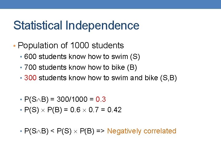
Statistical Independence • Population of 1000 students • 600 students know how to swim (S) • 700 students know how to bike (B) • 300 students know how to swim and bike (S, B) • P(S B) = 300/1000 = 0. 3 • P(S) P(B) = 0. 6 0. 7 = 0. 42 • P(S B) < P(S) P(B) => Negatively correlated

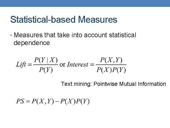
Statistical-based Measures • Measures that take into account statistical dependence Text mining: Pointwise Mutual Information

Example: Lift/Interest Coffee Tea 15 5 20 Tea 75 5 80 90 10 100 Association Rule: Tea Coffee Confidence= P(Coffee|Tea) = 0. 75 but P(Coffee) = 0. 9 Þ Lift = 0. 75/0. 9= 0. 8333 (< 1, therefore is negatively associated)

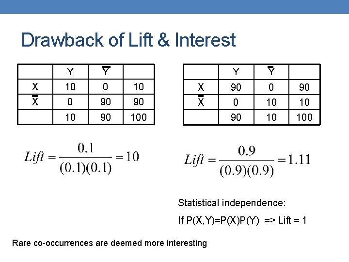
Drawback of Lift & Interest Y Y X 10 0 10 X 0 90 90 100 Y Y X 90 0 90 X 0 10 10 90 10 100 Statistical independence: If P(X, Y)=P(X)P(Y) => Lift = 1 Rare co-occurrences are deemed more interesting

ALTERNATIVE FREQUENT ITEMSET COMPUTATION Slides taken from Mining Massive Datasets course by Anand Rajaraman and Jeff Ullman.

Efficient computation of pairs • The operation that takes most resources (mostly in terms of memory, but also time) is the computation of frequent pairs. • How can we make this faster?

48 PCY Algorithm • During Pass 1 (computing frequent items) of A- priori, most memory is idle. • Use that memory to keep counts of buckets into which pairs of items are hashed. • Just the count, not the pairs themselves.

49 Needed Extensions Pairs of items need to be generated from the input file; they are not present in the file. 2. We are not just interested in the presence of a pair, but we need to see whether it is present at least s (support) times. 1.

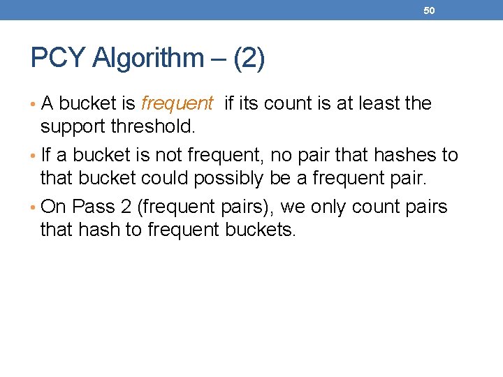
50 PCY Algorithm – (2) • A bucket is frequent if its count is at least the support threshold. • If a bucket is not frequent, no pair that hashes to that bucket could possibly be a frequent pair. • On Pass 2 (frequent pairs), we only count pairs that hash to frequent buckets.

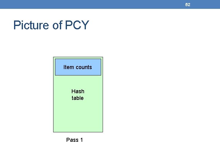
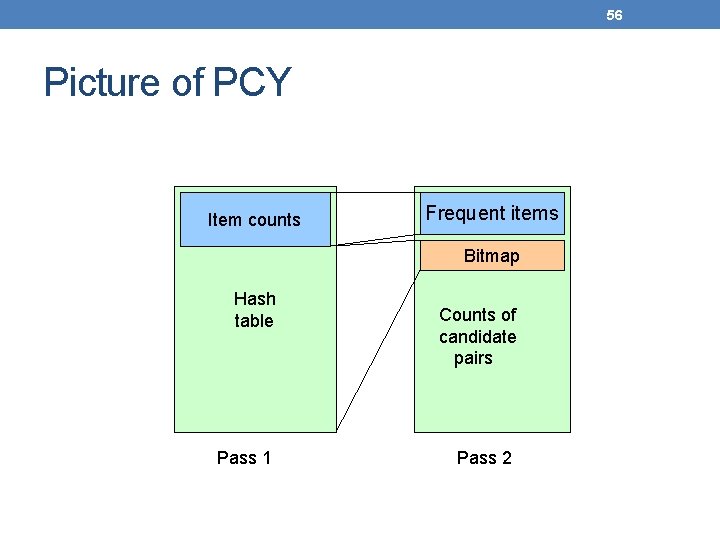
51 PCY Algorithm – Before Pass 1 Organize Main Memory • Space to count each item. • One (typically) 4 -byte integer per item. • Use the rest of the space for as many integers, representing buckets, as we can.

52 Picture of PCY Item counts Hash table Pass 1

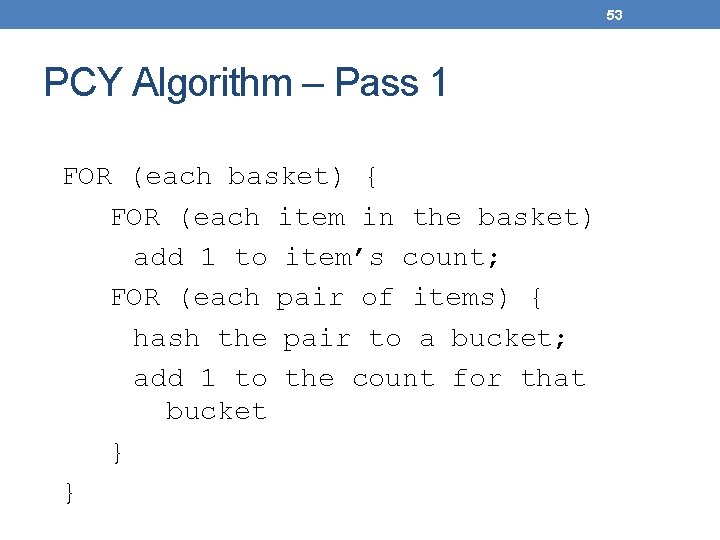
53 PCY Algorithm – Pass 1 FOR (each basket) { FOR (each item in the basket) add 1 to item’s count; FOR (each pair of items) { hash the pair to a bucket; add 1 to the count for that bucket } }

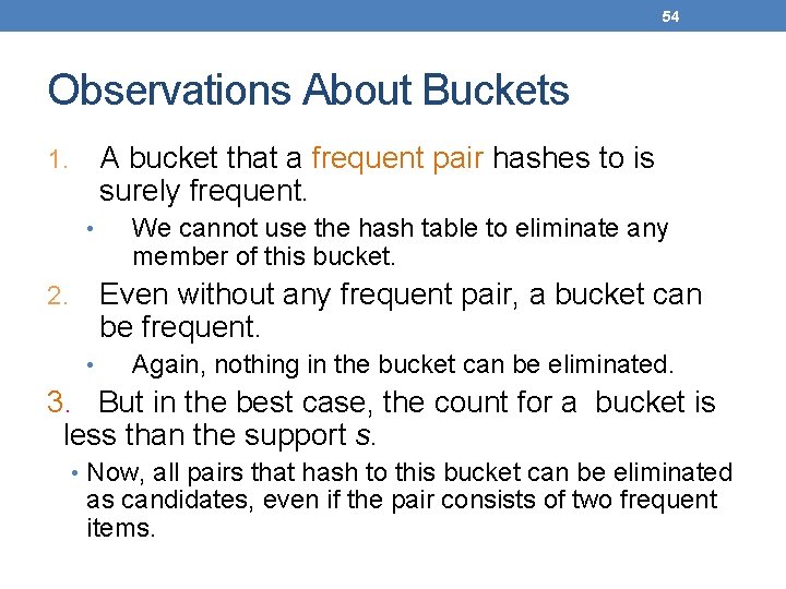
54 Observations About Buckets A bucket that a frequent pair hashes to is surely frequent. 1. • We cannot use the hash table to eliminate any member of this bucket. Even without any frequent pair, a bucket can be frequent. 2. • Again, nothing in the bucket can be eliminated. 3. But in the best case, the count for a bucket is less than the support s. • Now, all pairs that hash to this bucket can be eliminated as candidates, even if the pair consists of two frequent items.

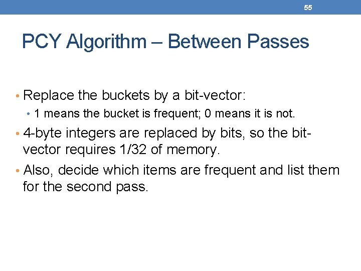
55 PCY Algorithm – Between Passes • Replace the buckets by a bit-vector: • 1 means the bucket is frequent; 0 means it is not. • 4 -byte integers are replaced by bits, so the bit- vector requires 1/32 of memory. • Also, decide which items are frequent and list them for the second pass.

56 Picture of PCY Item counts Frequent items Bitmap Hash table Pass 1 Counts of candidate pairs Pass 2

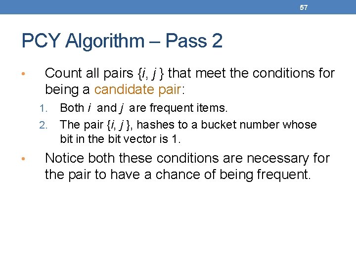
57 PCY Algorithm – Pass 2 • Count all pairs {i, j } that meet the conditions for being a candidate pair: 1. 2. • Both i and j are frequent items. The pair {i, j }, hashes to a bucket number whose bit in the bit vector is 1. Notice both these conditions are necessary for the pair to have a chance of being frequent.

58 All (Or Most) Frequent Itemsets In < 2 Passes • A-Priori, PCY, etc. , take k passes to find frequent itemsets of size k. • Other techniques use 2 or fewer passes for all sizes: • Simple sampling algorithm. • SON (Savasere, Omiecinski, and Navathe). • Toivonen.

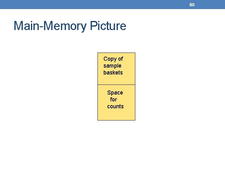
59 Simple Sampling Algorithm – (1) • Take a random sample of the market baskets. • Run a-priori or one of its improvements (for sets of all sizes, not just pairs) in main memory, so you don’t pay for disk I/O each time you increase the size of itemsets. • Be sure you leave enough space for counts.

60 Main-Memory Picture Copy of sample baskets Space for counts

61 Simple Algorithm – (2) • Use as your support threshold a suitable, scaled-back number. • E. g. , if your sample is 1/100 of the baskets, use s /100 as your support threshold instead of s.

62 Simple Algorithm – Option • Optionally, verify that your guesses are truly frequent in the entire data set by a second pass (eliminate false positives) • But you don’t catch sets frequent in the whole but not in the sample. (false negatives) • Smaller threshold, e. g. , s /125, helps catch more truly frequent itemsets. • But requires more space.

63 SON Algorithm – (1) • Repeatedly read small subsets of the baskets into main memory and perform the first pass of the simple algorithm on each subset. • An itemset becomes a candidate if it is found to be frequent in any one or more subsets of the baskets. • Threshold = s/number of subsets

64 SON Algorithm – (2) • On a second pass, count all the candidate itemsets and determine which are frequent in the entire set. • Key “monotonicity” idea: an itemset cannot be frequent in the entire set of baskets unless it is frequent in at least one subset. • Why?

65 SON Algorithm – Distributed Version • This idea lends itself to distributed data mining. • If baskets are distributed among many nodes, compute frequent itemsets at each node, then distribute the candidates from each node. • Finally, accumulate the counts of all candidates.

66 Toivonen’s Algorithm – (1) • Start as in the simple sampling algorithm, but lower the threshold slightly for the sample. • Example: if the sample is 1% of the baskets, use s /125 as the support threshold rather than s /100. • Goal is to avoid missing any itemset that is frequent in the full set of baskets.

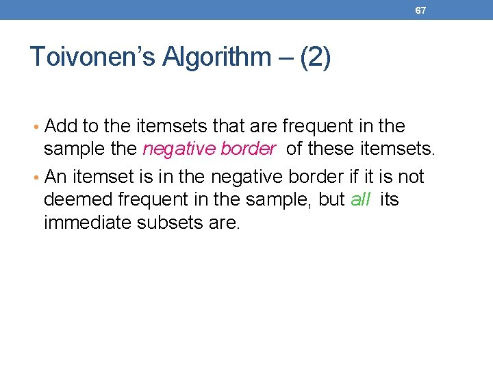
67 Toivonen’s Algorithm – (2) • Add to the itemsets that are frequent in the sample the negative border of these itemsets. • An itemset is in the negative border if it is not deemed frequent in the sample, but all its immediate subsets are.

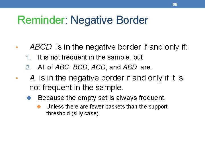
68 Reminder: Negative Border • ABCD is in the negative border if and only if: 1. 2. • It is not frequent in the sample, but All of ABC, BCD, ACD, and ABD are. A is in the negative border if and only if it is not frequent in the sample. u Because the empty set is always frequent. u Unless there are fewer baskets than the support threshold (silly case).

Negative Border Itemsets that are not frequent, but all their immediate subsets are frequent. Infrequent Itemsets Border

70 Picture of Negative Border … triples pairs singletons Frequent Itemsets from Sample

71 Toivonen’s Algorithm – (3) • In a second pass, count all candidate frequent itemsets from the first pass, and also count their negative border. • If no itemset from the negative border turns out to be frequent, then the candidates found to be frequent in the whole data are exactly the frequent itemsets.

72 Toivonen’s Algorithm – (4) • What if we find that something in the negative border is actually frequent? • We must start over again! • Try to choose the support threshold so the probability of failure is low, while the number of itemsets checked on the second pass fits in mainmemory.

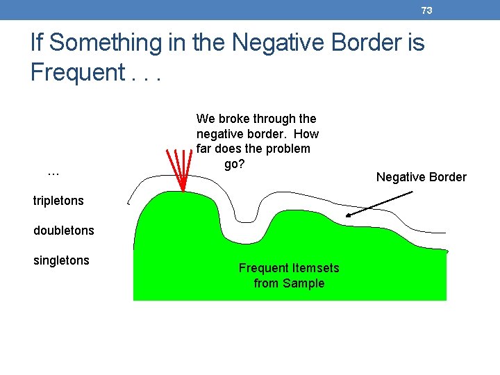
73 If Something in the Negative Border is Frequent. . . … We broke through the negative border. How far does the problem go? tripletons doubletons singletons Frequent Itemsets from Sample Negative Border

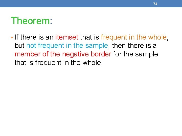
74 Theorem: • If there is an itemset that is frequent in the whole, but not frequent in the sample, then there is a member of the negative border for the sample that is frequent in the whole.

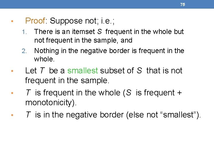
75 • Proof: Suppose not; i. e. ; 1. 2. • • • There is an itemset S frequent in the whole but not frequent in the sample, and Nothing in the negative border is frequent in the whole. Let T be a smallest subset of S that is not frequent in the sample. T is frequent in the whole (S is frequent + monotonicity). T is in the negative border (else not “smallest”).

Example Infrequent Itemsets Border

THE FP-TREE AND THE FP -GROWTH ALGORITHM Slides from course lecture of E. Pitoura

Overview • The FP-tree contains a compressed representation of the transaction database. • A trie (prefix-tree) data structure is used • Each transaction is a path in the tree – paths can overlap. • Once the FP-tree is constructed the recursive, divide-and-conquer FP-Growth algorithm is used to enumerate all frequent itemsets.

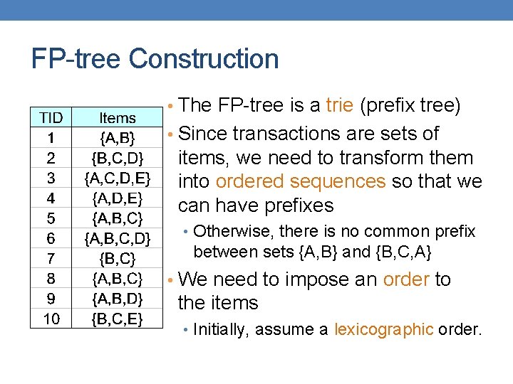
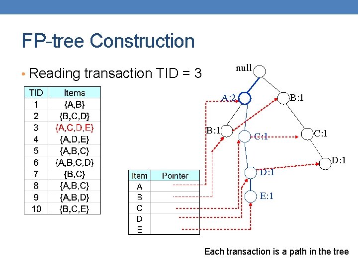
FP-tree Construction • The FP-tree is a trie (prefix tree) • Since transactions are sets of items, we need to transform them into ordered sequences so that we can have prefixes • Otherwise, there is no common prefix between sets {A, B} and {B, C, A} • We need to impose an order to the items • Initially, assume a lexicographic order.

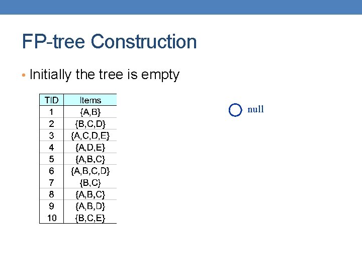
FP-tree Construction • Initially the tree is empty null

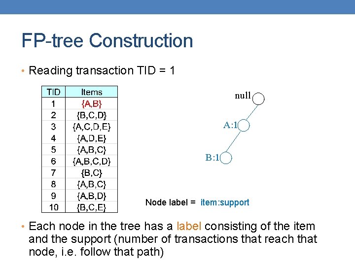
FP-tree Construction • Reading transaction TID = 1 null A: 1 B: 1 Node label = item: support • Each node in the tree has a label consisting of the item and the support (number of transactions that reach that node, i. e. follow that path)

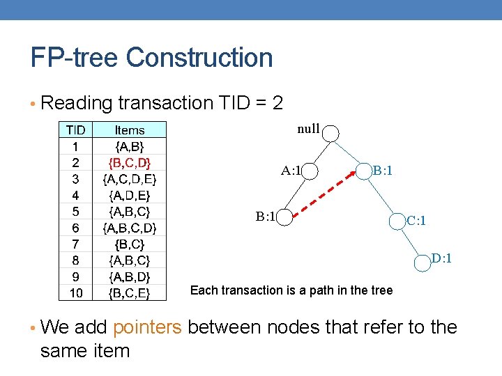
FP-tree Construction • Reading transaction TID = 2 null A: 1 B: 1 C: 1 D: 1 Each transaction is a path in the tree • We add pointers between nodes that refer to the same item

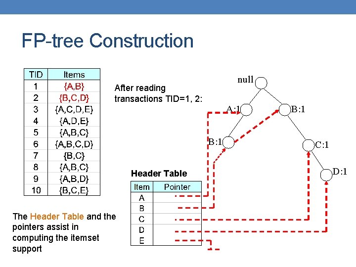
FP-tree Construction null After reading transactions TID=1, 2: A: 1 B: 1 Header Table The Header Table and the pointers assist in computing the itemset support B: 1 C: 1 D: 1

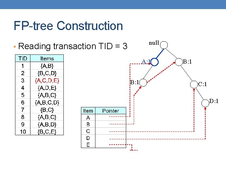
FP-tree Construction null • Reading transaction TID = 3 A: 1 B: 1 C: 1 D: 1

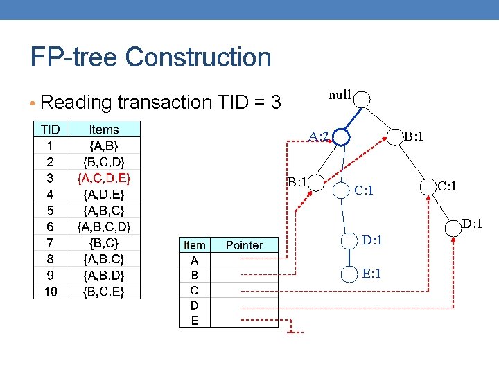
FP-tree Construction null • Reading transaction TID = 3 A: 2 B: 1 C: 1 D: 1 E: 1

FP-tree Construction null • Reading transaction TID = 3 A: 2 B: 1 C: 1 D: 1 E: 1 Each transaction is a path in the tree

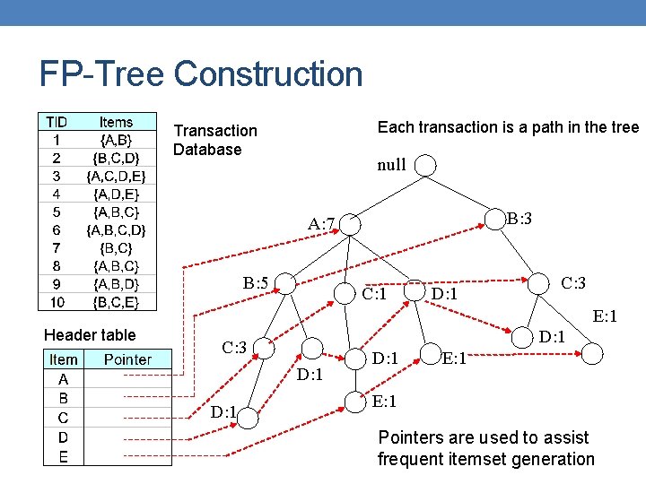
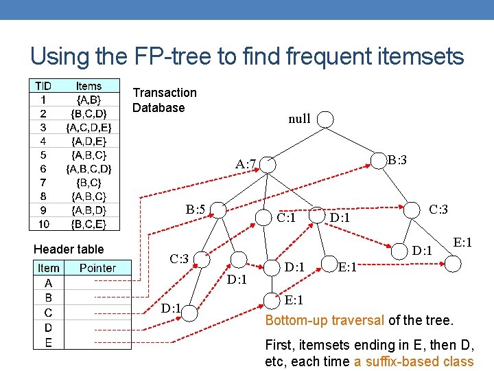
FP-Tree Construction Each transaction is a path in the tree Transaction Database null B: 3 A: 7 B: 5 C: 1 D: 1 C: 3 E: 1 Header table D: 1 C: 3 D: 1 E: 1 Pointers are used to assist frequent itemset generation

FP-tree size • Every transaction is a path in the FP-tree • The size of the tree depends on the compressibility of the data • Extreme case: All transactions are the same, the FP- tree is a single branch • Extreme case: All transactions are different the size of the tree is the same as that of the database (bigger actually since we need additional pointers)

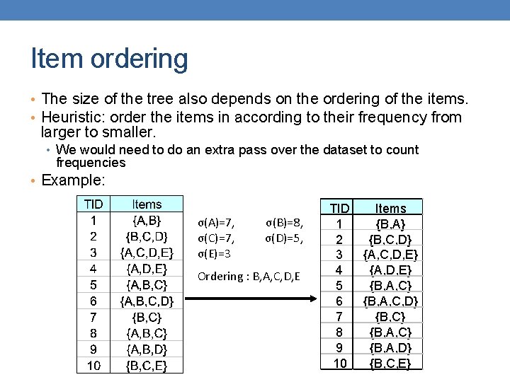
Item ordering • The size of the tree also depends on the ordering of the items. • Heuristic: order the items in according to their frequency from larger to smaller. • We would need to do an extra pass over the dataset to count frequencies • Example: σ(Α)=7, σ(C)=7, σ(Ε)=3 σ(Β)=8, σ(D)=5, Ordering : Β, Α, C, D, E TID 1 2 3 4 5 6 7 8 9 10 Items {Β, Α} {B, C, D} {A, C, D, E} {A, D, E} {Β, Α, C, D} {B, C} {Β, Α, D} {B, C, E}

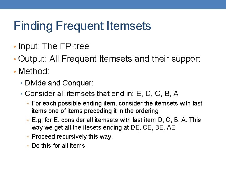
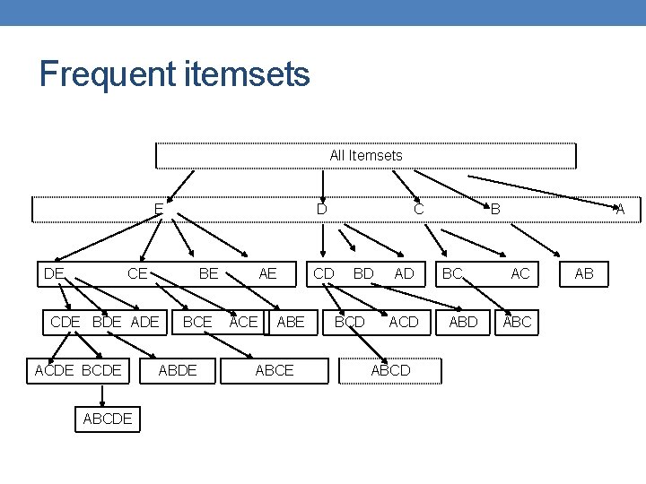
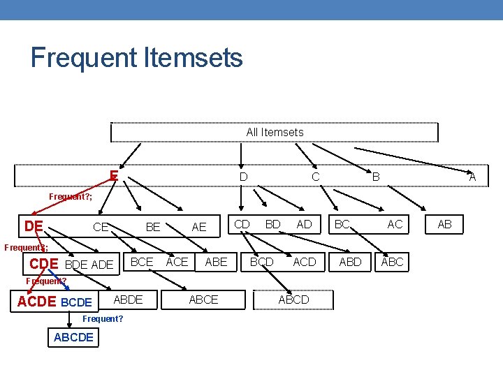
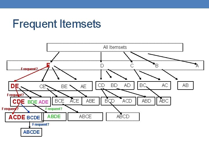
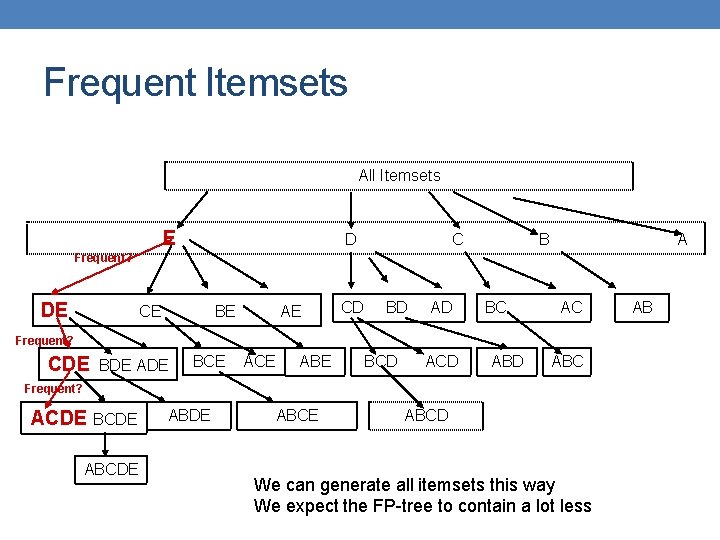
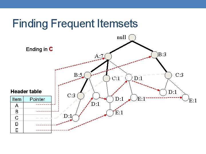
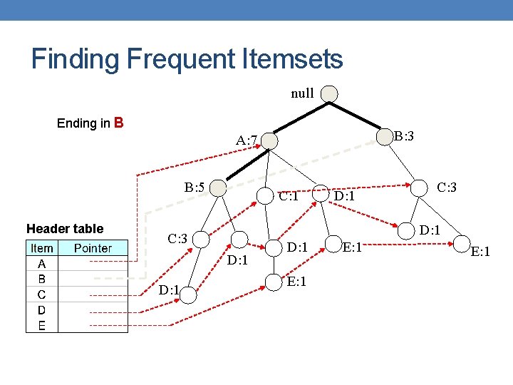
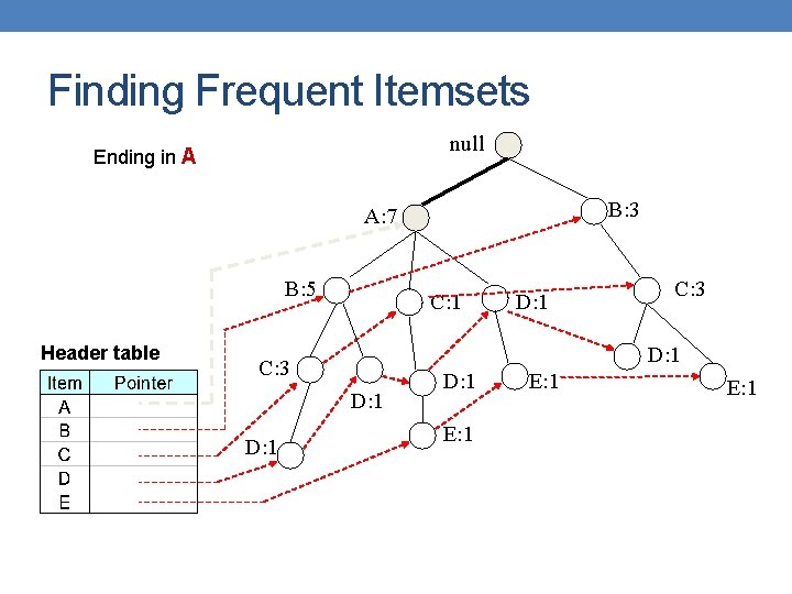
Finding Frequent Itemsets • Input: The FP-tree • Output: All Frequent Itemsets and their support • Method: • Divide and Conquer: • Consider all itemsets that end in: E, D, C, B, A • For each possible ending item, consider the itemsets with last items one of items preceding it in the ordering • E. g, for E, consider all itemsets with last item D, C, B, A. This way we get all the itesets ending at DE, CE, BE, AE • Proceed recursively this way. • Do this for all items.

Frequent itemsets All Itemsets Ε DE D CE BE CDE BDE ACDE BCDE ABCDE BCE ABDE AE ACE ABCE CD C BD BCD AD ACD ABCD B BC ABD A AC AB

Frequent Itemsets All Itemsets Ε D C B A Frequent? ; DE CE BE AE CD BD AD BC AC Frequent? ; CDE BDE ADE BCE ABE BCD ACD Frequent? ACDE BCDE ABDE Frequent? ABCDE ABCD ABC AB

Frequent Itemsets All Itemsets Ε Frequent? DE D CE BE AE CD C BD AD B BC A AC Frequent? CDE BDE ADE Frequent? BCE ABE BCD ACD Frequent? ACDE BCDE ABDE Frequent? ABCDE ABCD ABC AB

Frequent Itemsets All Itemsets Ε D C B A Frequent? DE CE BE AE CD BD AD BC AC Frequent? CDE BDE ADE BCE ABE BCD ABD ABC Frequent? ACDE BCDE ABDE ABCD We can generate all itemsets this way We expect the FP-tree to contain a lot less AB

Using the FP-tree to find frequent itemsets Transaction Database null B: 3 A: 7 B: 5 Header table C: 1 C: 3 D: 1 D: 1 E: 1 Bottom-up traversal of the tree. First, itemsets ending in E, then D, etc, each time a suffix-based class

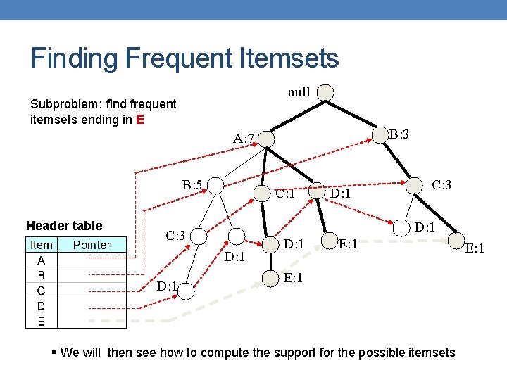
Finding Frequent Itemsets null Subproblem: find frequent itemsets ending in E B: 3 A: 7 B: 5 Header table C: 1 C: 3 D: 1 D: 1 E: 1 § We will then see how to compute the support for the possible itemsets E: 1

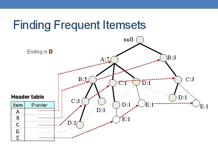
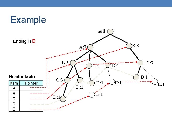
Finding Frequent Itemsets null Ending in D B: 3 A: 7 B: 5 Header table C: 1 C: 3 D: 1 D: 1 E: 1

Finding Frequent Itemsets null Ending in C B: 3 A: 7 B: 5 Header table C: 1 C: 3 D: 1 D: 1 E: 1

Finding Frequent Itemsets null Ending in B B: 3 A: 7 B: 5 Header table C: 1 C: 3 D: 1 D: 1 E: 1

Finding Frequent Itemsets null Ending in Α B: 3 A: 7 B: 5 Header table C: 1 C: 3 D: 1 D: 1 E: 1

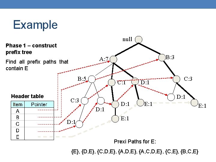
Algorithm • For each suffix X • Phase 1 • Construct the prefix tree for X as shown before, and compute the support using the header table and the pointers • Phase 2 • If X is frequent, construct the conditional FP-tree for X in the following steps 1. 2. 3. Recompute support Prune infrequent items Prune leaves and recurse

Example null Phase 1 – construct prefix tree Find all prefix paths that contain E B: 5 Header table B: 3 A: 7 C: 1 C: 3 D: 1 D: 1 E: 1 Prexi Paths for Ε: {E}, {D, E}, {C, D, E}, {A, D, Ε}, {A, C, D, E}, {C, E}, {B, C, E}

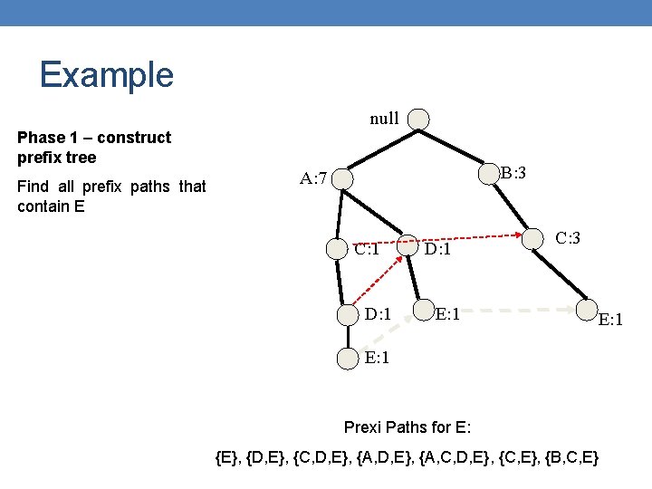
Example null Phase 1 – construct prefix tree Find all prefix paths that contain E B: 3 A: 7 C: 1 D: 1 E: 1 C: 3 E: 1 Prexi Paths for Ε: {E}, {D, E}, {C, D, E}, {A, D, Ε}, {A, C, D, E}, {C, E}, {B, C, E}

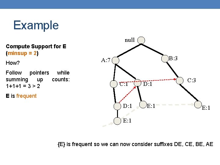
Example null Compute Support for E (minsup = 2) B: 3 A: 7 How? Follow pointers while summing up counts: 1+1+1 = 3 > 2 C: 1 D: 1 C: 3 E is frequent D: 1 E: 1 {E} is frequent so we can now consider suffixes DE, CE, BE, AE

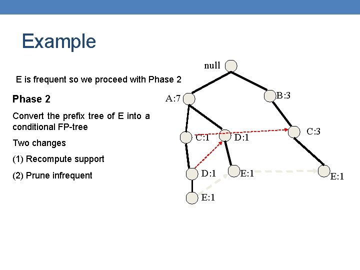
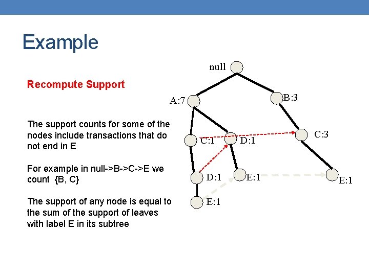
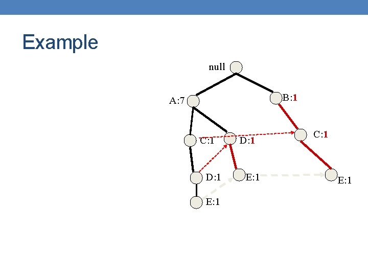
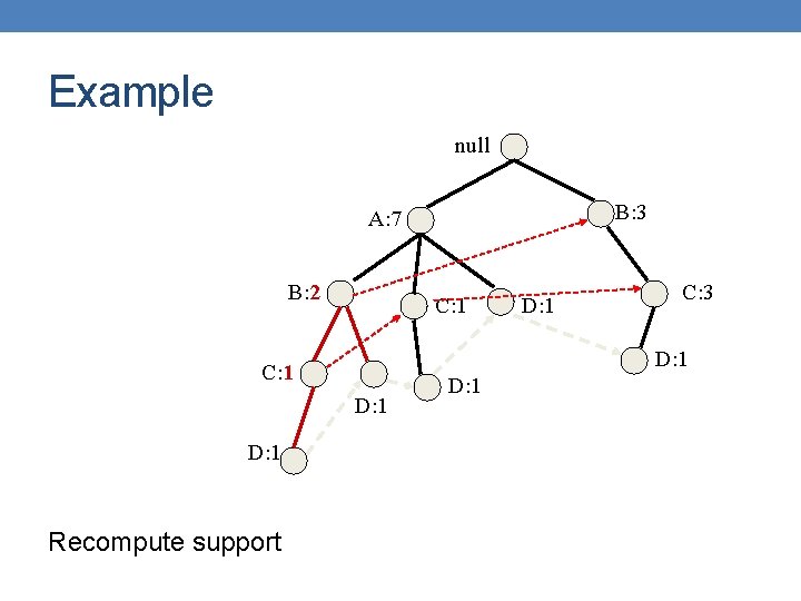
Example null E is frequent so we proceed with Phase 2 Convert the prefix tree of E into a conditional FP-tree Two changes B: 3 A: 7 C: 1 D: 1 C: 3 (1) Recompute support (2) Prune infrequent D: 1 E: 1

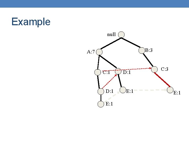
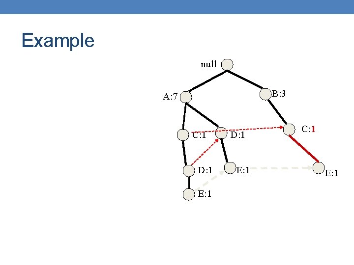
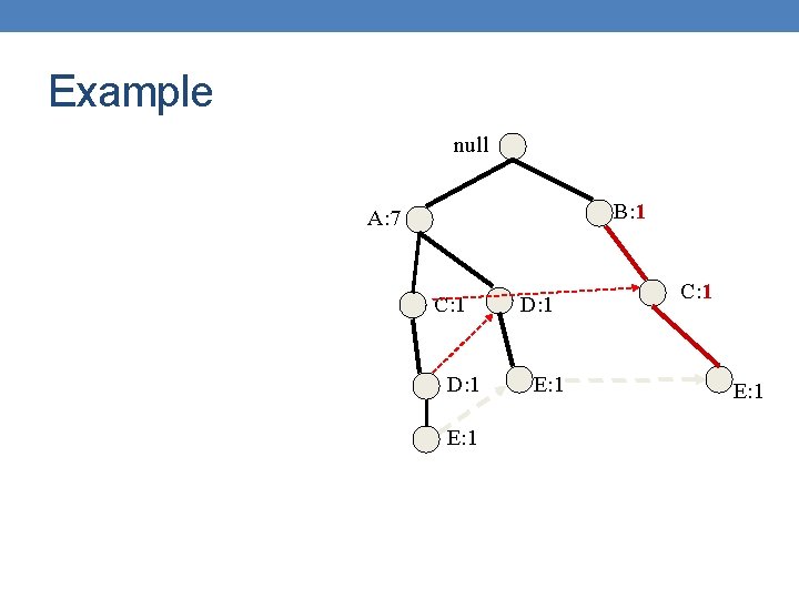
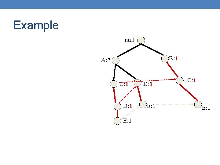
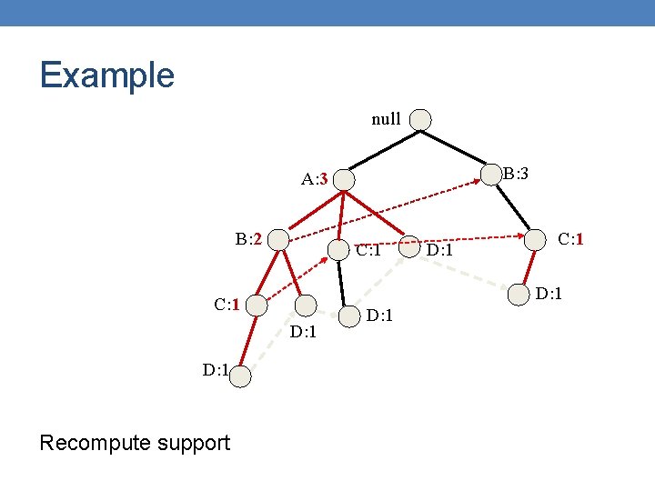
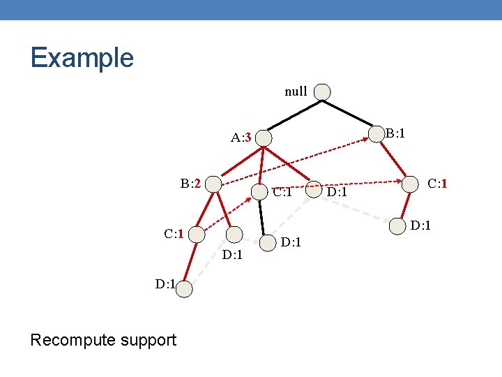
Example null Recompute Support B: 3 A: 7 The support counts for some of the nodes include transactions that do not end in E For example in null->B->C->E we count {B, C} The support of any node is equal to the sum of the support of leaves with label E in its subtree C: 1 D: 1 E: 1 C: 3 E: 1

Example null B: 3 A: 7 C: 1 D: 1 E: 1 C: 3 E: 1

Example null B: 3 A: 7 C: 1 D: 1 E: 1 C: 1 E: 1

Example null B: 1 A: 7 C: 1 D: 1 E: 1 C: 1 E: 1

Example null B: 1 A: 7 C: 1 D: 1 E: 1 C: 1 E: 1

Example null B: 1 A: 7 C: 1 D: 1 E: 1 C: 1 E: 1

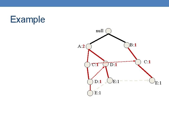
Example null B: 1 A: 2 C: 1 D: 1 E: 1 C: 1 E: 1

Example null B: 1 A: 2 C: 1 D: 1 E: 1 C: 1 E: 1

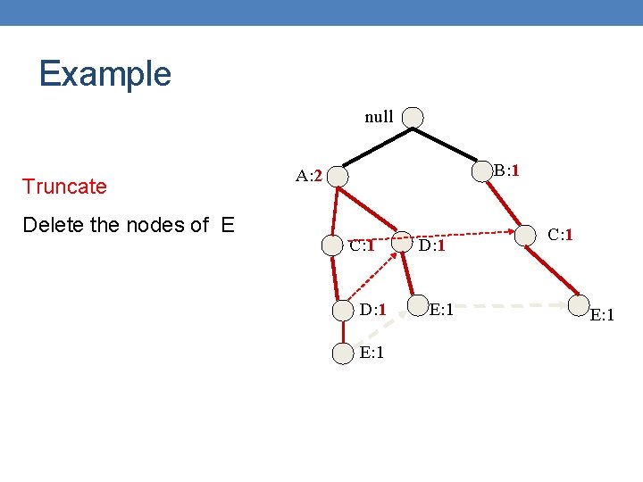
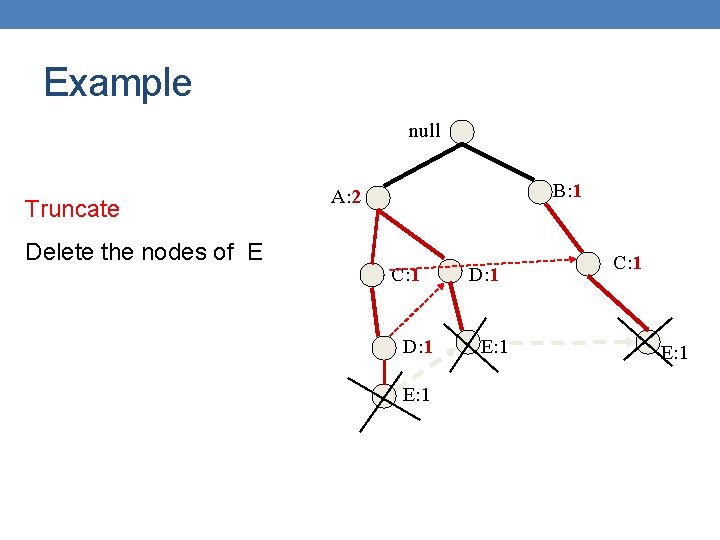
Example null Truncate Delete the nodes of Ε B: 1 A: 2 C: 1 D: 1 E: 1 C: 1 E: 1

Example null Truncate Delete the nodes of Ε B: 1 A: 2 C: 1 D: 1 E: 1 C: 1 E: 1

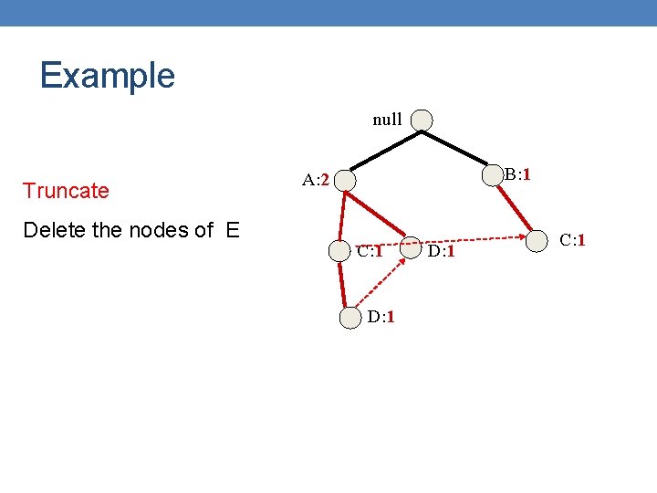
Example null Truncate Delete the nodes of Ε B: 1 A: 2 C: 1 D: 1 C: 1

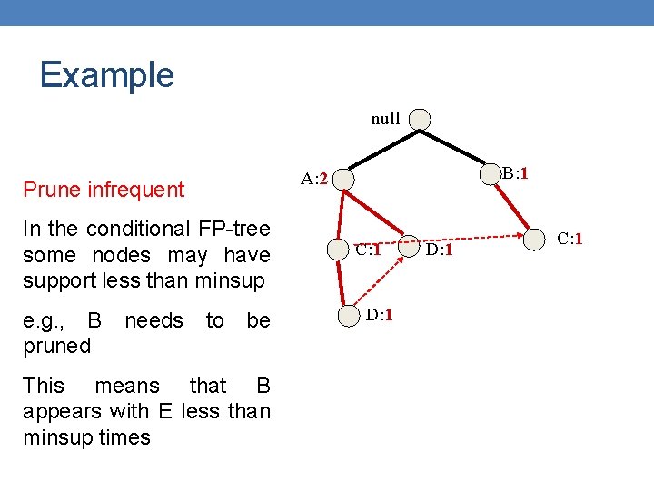
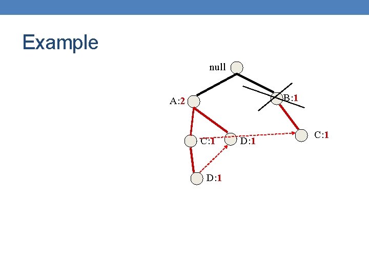
Example null Prune infrequent In the conditional FP-tree some nodes may have support less than minsup e. g. , B pruned needs B: 1 A: 2 to be This means that B appears with E less than minsup times C: 1 D: 1 C: 1

Example null B: 1 A: 2 C: 1 D: 1 C: 1

Example null C: 1 A: 2 C: 1 D: 1

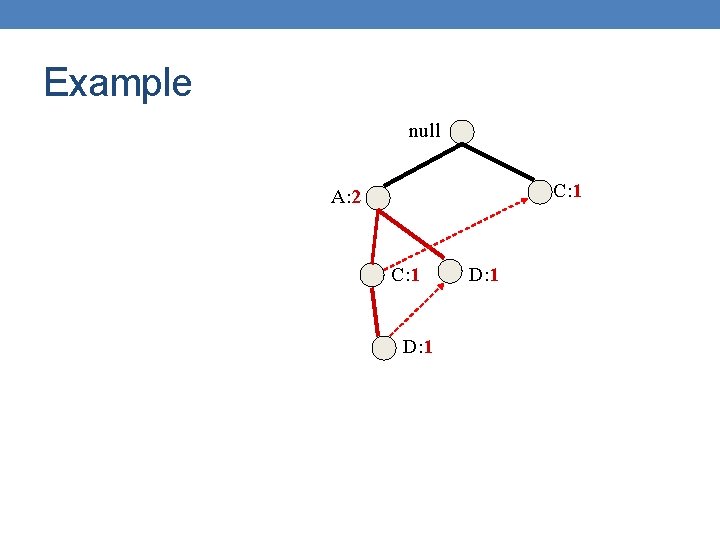
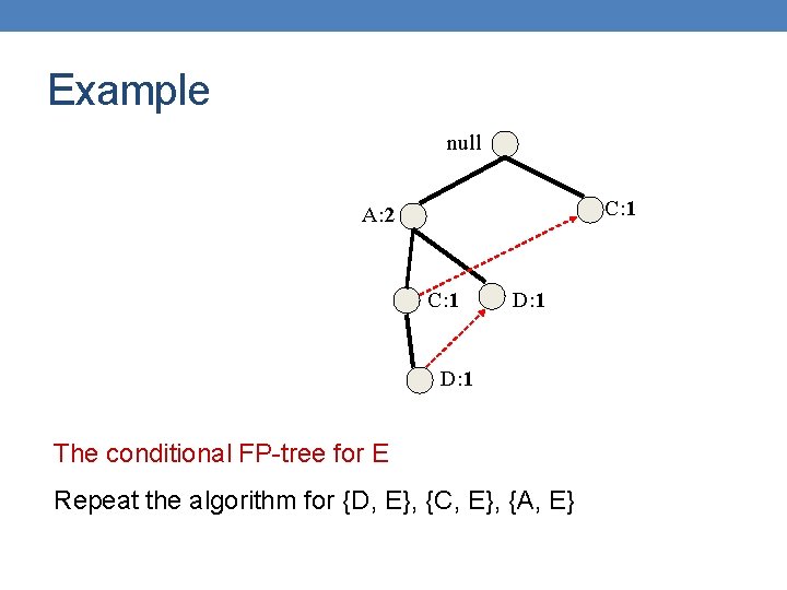
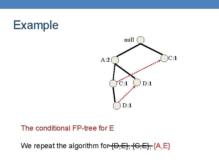
Example null C: 1 A: 2 C: 1 D: 1 The conditional FP-tree for E Repeat the algorithm for {D, E}, {C, E}, {A, E}

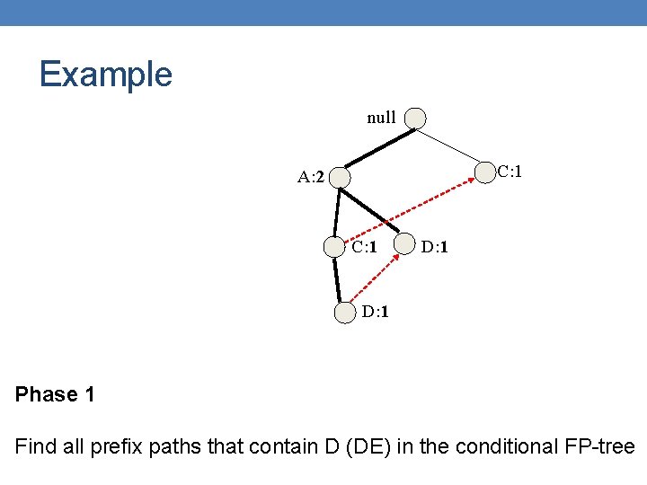
Example null C: 1 A: 2 C: 1 D: 1 Phase 1 Find all prefix paths that contain D (DE) in the conditional FP-tree

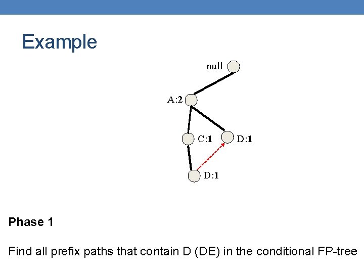
Example null A: 2 C: 1 D: 1 Phase 1 Find all prefix paths that contain D (DE) in the conditional FP-tree

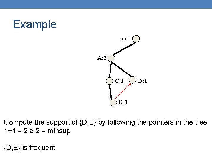
Example null A: 2 C: 1 D: 1 Compute the support of {D, E} by following the pointers in the tree 1+1 = 2 ≥ 2 = minsup {D, E} is frequent

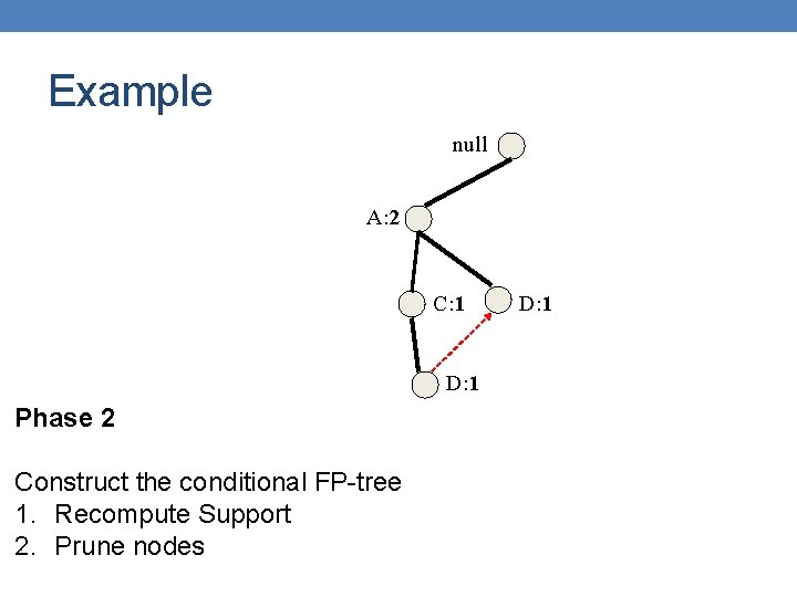
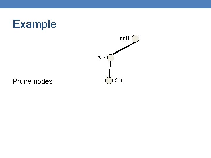
Example null A: 2 C: 1 D: 1 Phase 2 Construct the conditional FP-tree 1. Recompute Support 2. Prune nodes D: 1

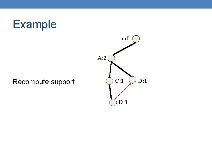
Example null A: 2 Recompute support C: 1 D: 1

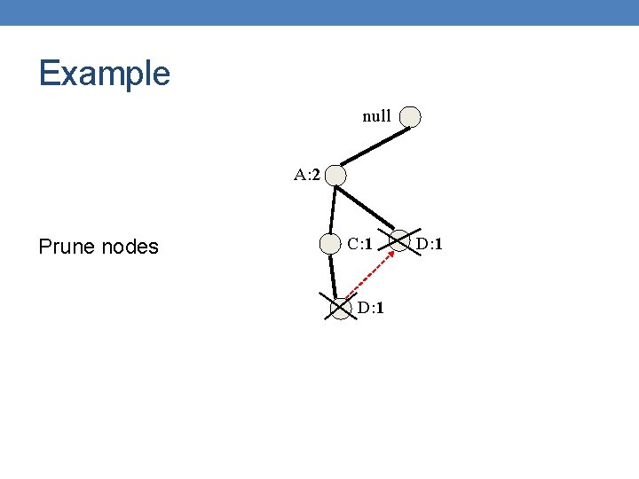
Example null A: 2 Prune nodes C: 1 D: 1

Example null A: 2 Prune nodes C: 1

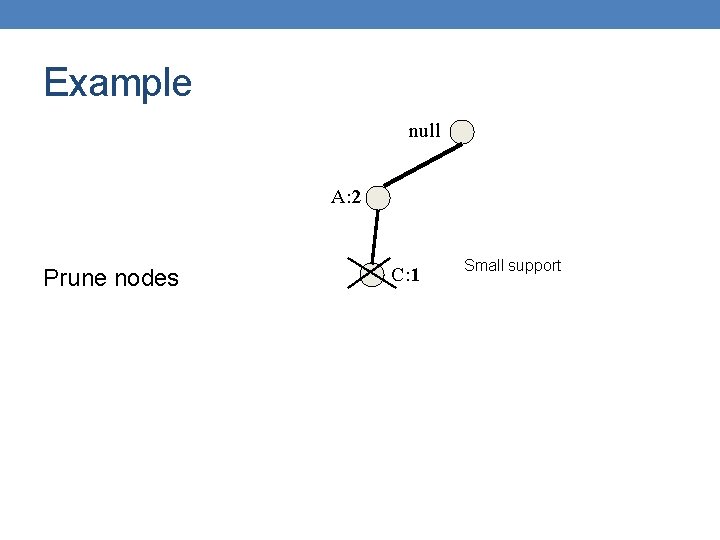
Example null A: 2 Prune nodes C: 1 Small support

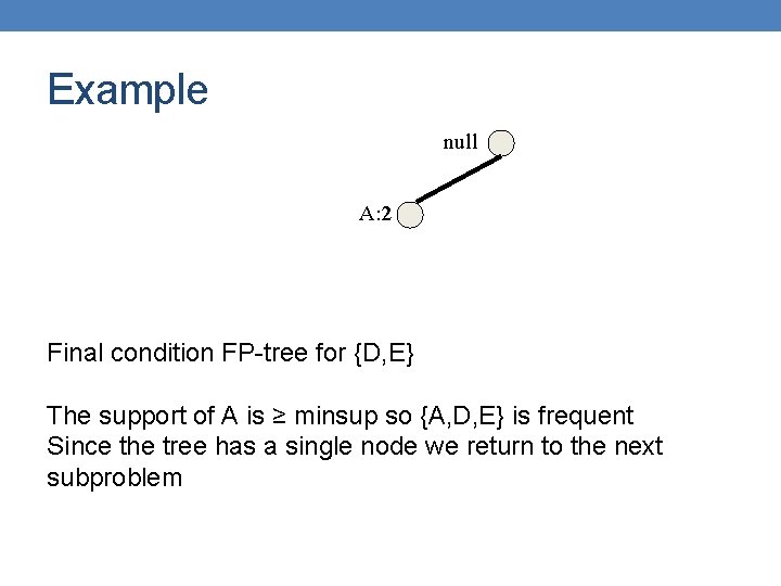
Example null A: 2 Final condition FP-tree for {D, E} The support of A is ≥ minsup so {A, D, E} is frequent Since the tree has a single node we return to the next subproblem

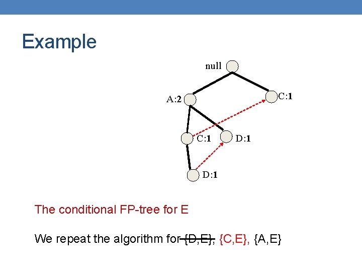
Example null C: 1 A: 2 C: 1 D: 1 The conditional FP-tree for E We repeat the algorithm for {D, E}, {C, E}, {A, E}

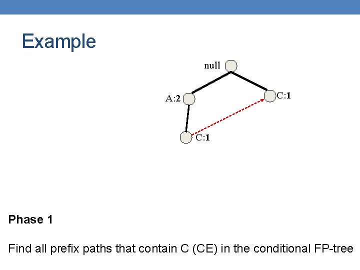
Example null C: 1 A: 2 C: 1 D: 1 Phase 1 Find all prefix paths that contain C (CE) in the conditional FP-tree

Example null C: 1 A: 2 C: 1 Phase 1 Find all prefix paths that contain C (CE) in the conditional FP-tree

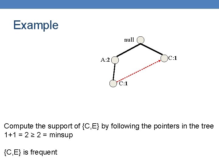
Example null C: 1 A: 2 C: 1 Compute the support of {C, E} by following the pointers in the tree 1+1 = 2 ≥ 2 = minsup {C, E} is frequent

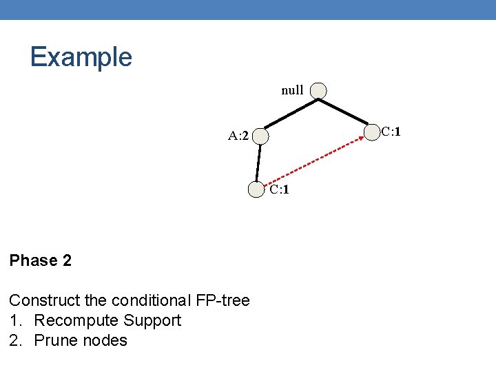
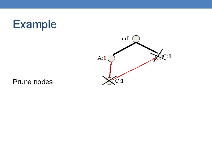
Example null C: 1 A: 2 C: 1 Phase 2 Construct the conditional FP-tree 1. Recompute Support 2. Prune nodes

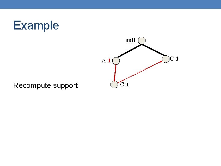
Example null C: 1 A: 1 Recompute support C: 1

Example null C: 1 A: 1 Prune nodes C: 1

Example null A: 1 Prune nodes

Example null A: 1 Prune nodes

Example null Prune nodes Return to the previous subproblem

Example null C: 1 A: 2 C: 1 D: 1 The conditional FP-tree for E We repeat the algorithm for {D, E}, {C, E}, {A, E}

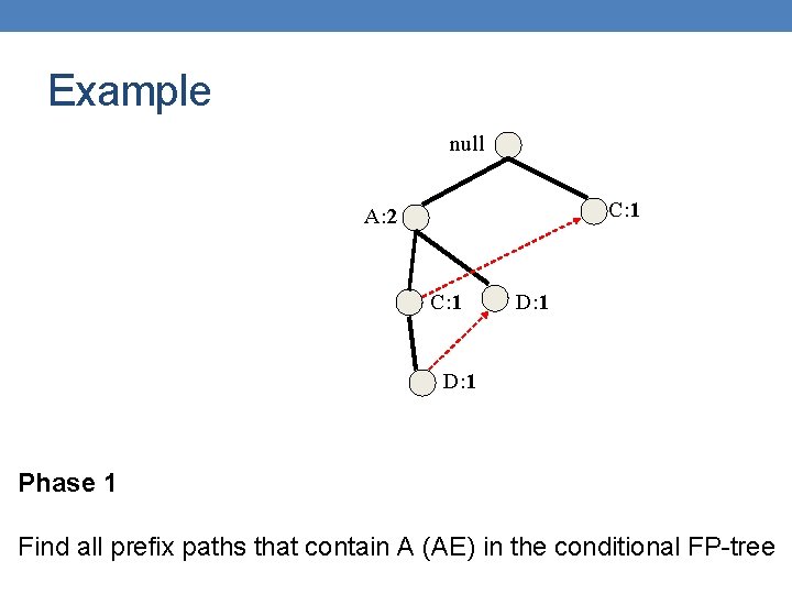
Example null C: 1 A: 2 C: 1 D: 1 Phase 1 Find all prefix paths that contain A (AE) in the conditional FP-tree

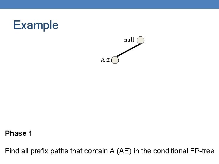
Example null A: 2 Phase 1 Find all prefix paths that contain A (AE) in the conditional FP-tree

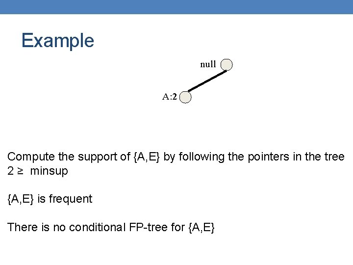
Example null A: 2 Compute the support of {A, E} by following the pointers in the tree 2 ≥ minsup {A, E} is frequent There is no conditional FP-tree for {A, E}

Example • So for E we have the following frequent itemsets {E}, {D, E}, {C, E}, {A, E} • We proceed with D

Example null Ending in D B: 3 A: 7 B: 5 Header table C: 1 C: 3 D: 1 D: 1 E: 1

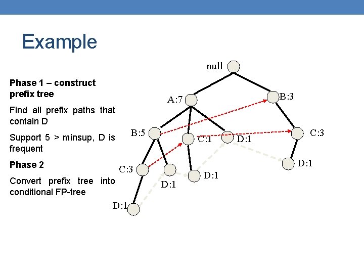
Example null Phase 1 – construct prefix tree B: 3 A: 7 Find all prefix paths that contain D B: 5 Support 5 > minsup, D is frequent Phase 2 C: 1 D: 1 C: 3 Convert prefix tree into conditional FP-tree D: 1

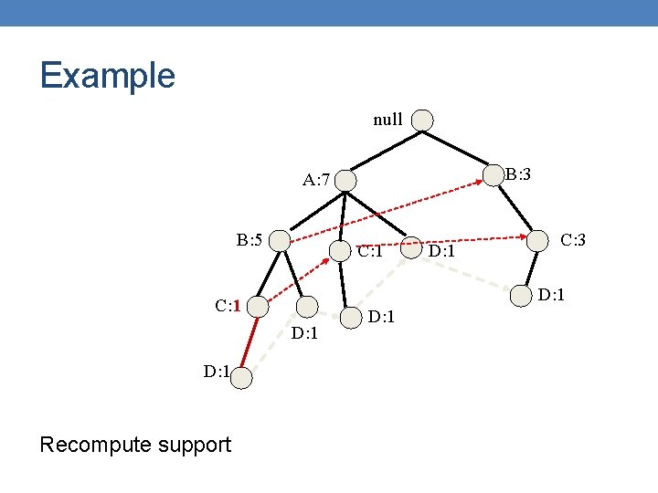
Example null B: 3 A: 7 B: 5 C: 1 D: 1 Recompute support C: 3 D: 1 C: 1 D: 1

Example null B: 3 A: 7 B: 2 C: 1 D: 1 Recompute support C: 3 D: 1 C: 1 D: 1

Example null B: 3 A: 3 B: 2 C: 1 D: 1 Recompute support C: 3 D: 1 C: 1 D: 1

Example null B: 3 A: 3 B: 2 C: 1 D: 1 Recompute support C: 1 D: 1

Example null B: 1 A: 3 B: 2 C: 1 D: 1 Recompute support C: 1 D: 1

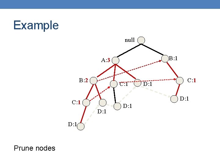
Example null B: 1 A: 3 B: 2 C: 1 D: 1 Prune nodes C: 1 D: 1

Example null B: 1 A: 3 B: 2 C: 1 Prune nodes C: 1

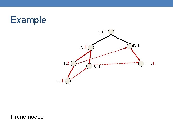
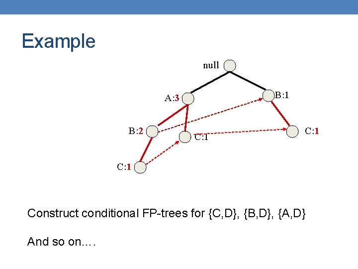
Example null B: 1 A: 3 B: 2 C: 1 Construct conditional FP-trees for {C, D}, {B, D}, {A, D} And so on….

Observations • At each recursive step we solve a subproblem • Construct the prefix tree • Compute the new support • Prune nodes • Subproblems are disjoint so we never consider the same itemset twice • Support computation is efficient – happens together with the computation of the frequent itemsets.

Observations • The efficiency of the algorithm depends on the compaction factor of the dataset • If the tree is bushy then the algorithm does not work well, it increases a lot of number of subproblems that need to be solved.

FREQUENT ITEMSET RESEARCH