Frequent Itemsets The MarketBasket Model Association Rules APriori

Frequent Itemsets The Market-Basket Model Association Rules A-Priori Algorithm Other Algorithms Jeffrey D. Ullman Stanford University

The Market-Basket Model �A large set of items, e. g. , things sold in a supermarket. �A large set of baskets, each of which is a small set of the items, e. g. , the things one customer buys on one day. 2

Support �Simplest question: find sets of items that appear “frequently” in the baskets. �Support for itemset I = the number of baskets containing all items in I. § Sometimes given as a percentage of the baskets. �Given a support threshold s, a set of items appearing in at least s baskets is called a frequent itemset. 3

Example: Frequent Itemsets �Items={milk, coke, pepsi, beer, juice}. �Support = 3 baskets. B 1 = {m, c, b} B 3 = {m, b} B 5 = {m, p, b} B 7 = {c, b, j} B 2 = {m, p, j} B 4 = {c, j} B 6 = {m, c, b, j} B 8 = {b, c} �Frequent itemsets: {m}, {c}, {b}, {j}, {m, b}, {b, c}, {c, j}. 4

Applications �“Classic” application was analyzing what people bought together in a brick-and-mortar store. § Apocryphal story of “diapers and beer” discovery. § Used to position potato chips between diapers and beer to enhance sales of potato chips. �Many other applications, including plagiarism detection. § Items = documents; baskets = sentences. § Basket/sentence contains all the items/documents that have that sentence. 5

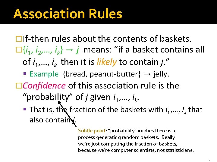
Association Rules �If-then rules about the contents of baskets. �{i 1, i 2, …, ik} → j means: “if a basket contains all of i 1, …, ik then it is likely to contain j. ” § Example: {bread, peanut-butter} → jelly. �Confidence of this association rule is the “probability” of j given i 1, …, ik. § That is, the fraction of the baskets with i 1, …, ik that also contain j. Subtle point: “probability” implies there is a process generating random baskets. Really we’re just computing the fraction of baskets, because we’re computer scientists, not statisticians. 6

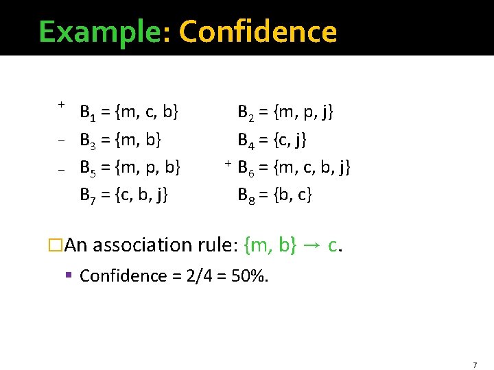
Example: Confidence + _ _ B 1 = {m, c, b} B 3 = {m, b} B 5 = {m, p, b} B 7 = {c, b, j} B 2 = {m, p, j} B 4 = {c, j} + B = {m, c, b, j} 6 B 8 = {b, c} �An association rule: {m, b} → c. § Confidence = 2/4 = 50%. 7

Computation Model �Typically, data is a file consisting of a list of baskets. �The true cost of mining disk-resident data is usually the number of disk I/O’s. �In practice, we read the data in passes – all baskets read in turn. § Thus, we measure the cost by the number of passes an algorithm takes. 8

Main-Memory Bottleneck �For many frequent-itemset algorithms, main memory is the critical resource. �As we read baskets, we need to count something, e. g. , occurrences of pairs of items. �The number of different things we can count is limited by main memory. § Swapping counts in/out is a disaster. 9

Finding Frequent Pairs �The hardest problem often turns out to be finding the frequent pairs. § Why? Often frequent pairs are common, frequent triples are rare. § Why? Support threshold is usually set high enough that you don’t get too many frequent itemsets. �We’ll concentrate on pairs, then extend to larger sets. 10

Naïve Algorithm �Read file once, counting in main memory the occurrences of each pair. § From each basket of n items, generate its n(n-1)/2 pairs by two nested loops. �Fails if (#items)2 exceeds main memory. § Example: Walmart sells 100 K items, so probably OK. § Example: Web has 100 B pages, so definitely not OK. 11

2 Approaches to Main-Memory Counting 1. Count all pairs, using a triangular matrix. § § I. e. , count {i, j} in row i, column j, provided i < j. But use a “ragged array, ” so the empty triangle is not there. 2. Keep a table of triples [i, j, c] = “the count of the pair of items {i, j} is c. ” (1) requires only 4 bytes/pair. � § Note: always assume integers are 4 bytes. (2) requires at least 12 bytes/pair, but only for those pairs with count > 0. I. e. , (2) beats (1) only when at most 1/3 of all pairs have a nonzero count. 12

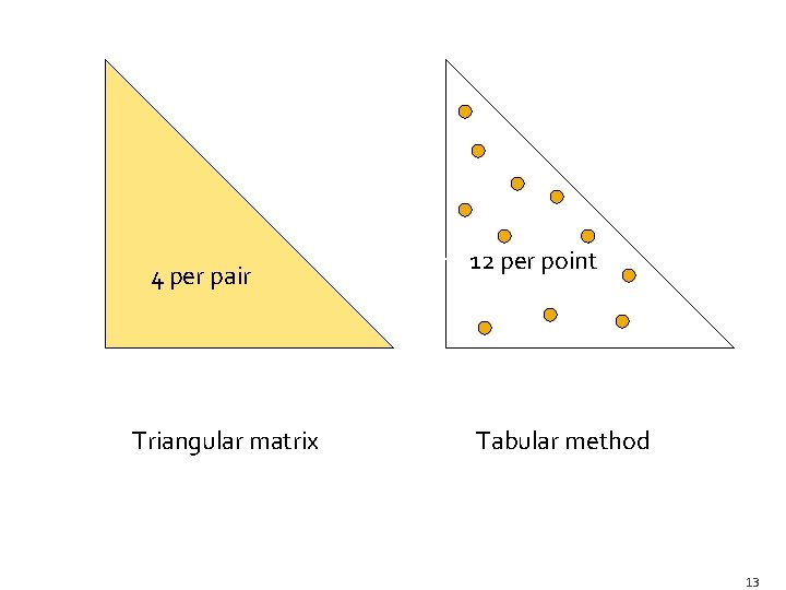
4 per pair Triangular matrix 1212 per point per occurring pair Tabular method 13

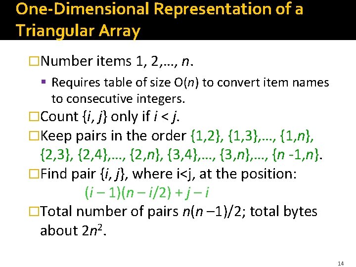
One-Dimensional Representation of a Triangular Array �Number items 1, 2, …, n. § Requires table of size O(n) to convert item names to consecutive integers. �Count {i, j} only if i < j. �Keep pairs in the order {1, 2}, {1, 3}, …, {1, n}, {2, 3}, {2, 4}, …, {2, n}, {3, 4}, …, {3, n}, …, {n -1, n}. �Find pair {i, j}, where i<j, at the position: (i – 1)(n – i/2) + j – i �Total number of pairs n(n – 1)/2; total bytes about 2 n 2. 14

The A-Priori Algorithm Monotonicity of “Frequent” Candidate Pairs Extension to Larger Itemsets

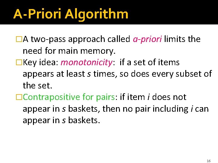
A-Priori Algorithm �A two-pass approach called a-priori limits the need for main memory. �Key idea: monotonicity: if a set of items appears at least s times, so does every subset of the set. �Contrapositive for pairs: if item i does not appear in s baskets, then no pair including i can appear in s baskets. 16

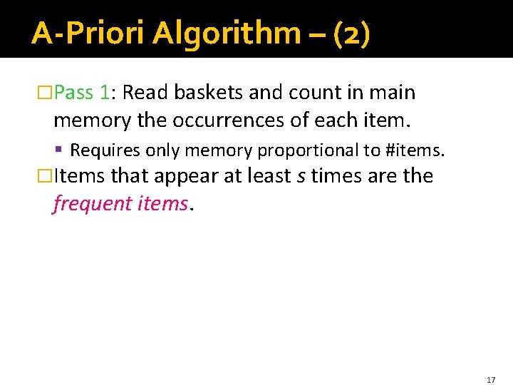
A-Priori Algorithm – (2) �Pass 1: Read baskets and count in main memory the occurrences of each item. § Requires only memory proportional to #items. �Items that appear at least s times are the frequent items. 17

A-Priori Algorithm – (3) �Pass 2: Read baskets again and count in main memory only those pairs both of which were found in Pass 1 to be frequent. �Requires memory proportional to square of frequent items only (for counts), plus a table of the frequent items (so you know what must be counted). 18

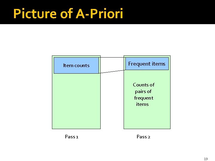
Picture of A-Priori Item counts Frequent items Counts of pairs of frequent items Pass 1 Pass 2 19

Detail for A-Priori �You can use the triangular matrix method with n = number of frequent items. § May save space compared with storing triples. �Trick: number frequent items 1, 2, … and keep a table relating new numbers to original item numbers. 20

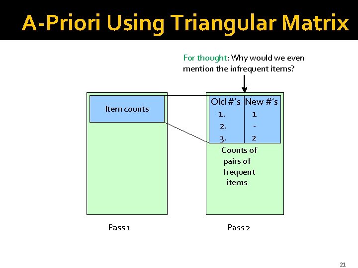
A-Priori Using Triangular Matrix For thought: Why would we even mention the infrequent items? Item counts Old #’s New #’s 1. 1 2. 3. 2 Counts of pairs of frequent items Pass 1 Pass 2 21

Frequent Triples, Etc. �For each size of itemsets k, we construct two sets of k-sets (sets of size k): § Ck = candidate k-sets = those that might be frequent sets (support > s) based on information from the pass for itemsets of size k – 1. § Lk = the set of truly frequent k-sets. 22

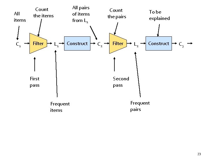
All items C 1 All pairs of items from L 1 Count the items Filter L 1 Construct First pass Count the pairs C 2 Filter To be explained L 2 Construct C 3 Second pass Frequent items Frequent pairs 23

Passes Beyond Two �C 1 = all items �In general, Lk = members of Ck with support ≥ s. § Requires one pass. �Ck+1 = (k+1)-sets, each k of which is in Lk. �For thought: how would you generate Ck+1 from Lk? § Enumerating all sets of size k+1 and testing each seems really dumb. 24

Memory Requirements �At the kth pass, you need space to count each member of Ck. �In realistic cases, because you need fairly high support, the number of candidates of each size drops, once you get beyond pairs. 25

The PCY (Park-Chen-Yu) Algorithm Improvement to A-Priori Exploits Empty Memory on First Pass Frequent Buckets

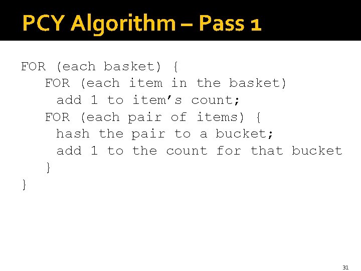
PCY Algorithm �During Pass 1 of A-priori, most memory is idle. �Use that memory to keep counts of buckets into which pairs of items are hashed. § Just the count, not the pairs themselves. �For each basket, enumerate all its pairs, hash them, and increment the resulting bucket count by 1. 27

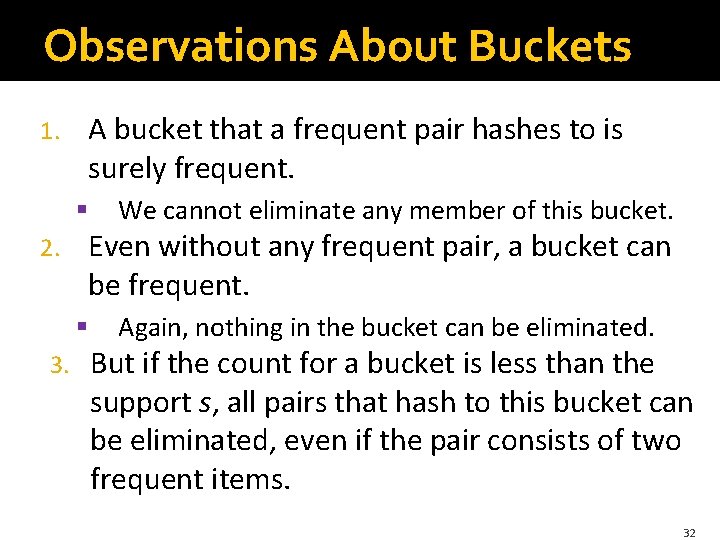
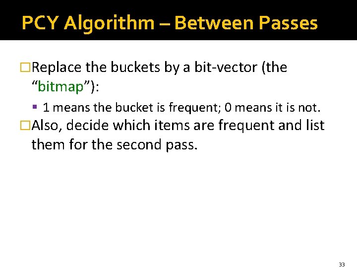
PCY Algorithm – (2) �A bucket is frequent if its count is at least the support threshold. �If a bucket is not frequent, no pair that hashes to that bucket could possibly be a frequent pair. �On Pass 2, we only count pairs of frequent items that also hash to a frequent bucket. �A bitmap tells which buckets are frequent, using only one bit per bucket (i. e. , 1/32 of the space used on Pass 1). 28

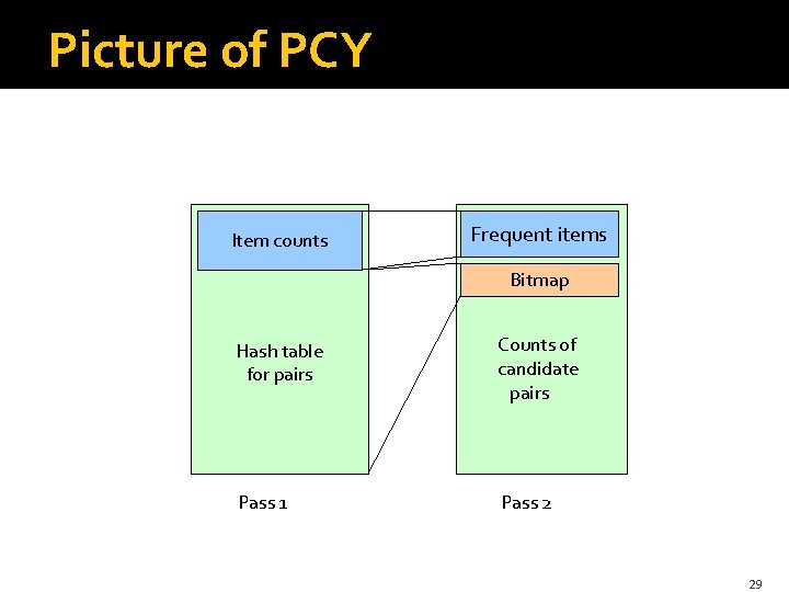
Picture of PCY Item counts Frequent items Bitmap Hash table for pairs Counts of candidate pairs Pass 1 Pass 2 29

Pass 1: Memory Organization �Space to count each item. § One (typically) 4 -byte integer per item. �Use the rest of the space for as many integers, representing buckets, as we can. 30

PCY Algorithm – Pass 1 FOR (each basket) { FOR (each item in the basket) add 1 to item’s count; FOR (each pair of items) { hash the pair to a bucket; add 1 to the count for that bucket } } 31

Observations About Buckets 1. A bucket that a frequent pair hashes to is surely frequent. § 2. Even without any frequent pair, a bucket can be frequent. § 3. We cannot eliminate any member of this bucket. Again, nothing in the bucket can be eliminated. But if the count for a bucket is less than the support s, all pairs that hash to this bucket can be eliminated, even if the pair consists of two frequent items. 32

PCY Algorithm – Between Passes �Replace the buckets by a bit-vector (the “bitmap”): § 1 means the bucket is frequent; 0 means it is not. �Also, decide which items are frequent and list them for the second pass. 33

PCY Algorithm – Pass 2 � Count all pairs {i, j} that meet the conditions for being a candidate pair: 1. Both i and j are frequent items. 2. The pair {i, j}, hashes to a bucket number whose bit in the bit vector is 1. 34

Memory Details �Buckets require a few bytes each. § Note: we don’t have to count past s. § If s < 216, 2 bytes/bucket will do. § # buckets is O(main-memory size). �On second pass, a table of (item, count) triples is essential. § Thus, hash table on Pass 1 must eliminate 2/3 of the candidate pairs for PCY to beat a-priori. 35

More Extensions to A-Priori �The MMDS book covers several other extensions beyond the PCY idea: “Multistage” and “Multihash. ” �For reading on your own, Sect. 6. 4 of MMDS. �Recommended video (starting about 10: 10): https: //www. youtube. com/watch? v=AGAk. Ni. Qnbj. Y 36

All (Or Most) Frequent Itemsets In < 2 Passes Simple Algorithm Savasere-Omiecinski- Navathe (SON) Algorithm Toivonen’s Algorithm

Simple Algorithm �Take a random sample of the market baskets. § Do not sneer; “random sample” is often a cure for the problem of having too large a dataset. �Run a-priori or one of its improvements (for sets of all sizes, not just pairs) in main memory, so you don’t pay for disk I/O each time you increase the size of itemsets. �Use as your support threshold a suitable, scaled-back number. § Example: if your sample is 1/100 of the baskets, use s/100 as your support threshold instead of s. 38

Simple Algorithm – Option �Optionally, verify that your guesses are truly frequent in the entire data set by a second pass. �But you don’t catch sets frequent in the whole but not in the sample. § Smaller threshold, e. g. , s/125 instead of s/100, helps catch more truly frequent itemsets. § But requires more space. 39

SON Algorithm �Partition the baskets into small subsets. �Read each subset into main memory and perform the first pass of the simple algorithm on each subset. § Parallel processing of the subsets a good option. �An itemset is a candidate if it is frequent (with support threshold suitably scaled down) in at least one subset. 40

SON Algorithm – Pass 2 �On a second pass, count all the candidate itemsets and determine which are frequent in the entire set. �Key “monotonicity” idea: an itemset cannot be frequent in the entire set of baskets unless it is frequent in at least one subset. 41

Toivonen’s Algorithm �Start as in the simple algorithm, but lower the threshold slightly for the sample. § Example: if the sample is 1% of the baskets, use s/125 as the support threshold rather than s/100. § Goal is to avoid missing any itemset that is frequent in the full set of baskets. 42

Toivonen’s Algorithm – (2) �Add to the itemsets that are frequent in the sample the negative border of these itemsets. �An itemset is in the negative border if it is not deemed frequent in the sample, but all its immediate subsets are. § Immediate subset = “delete exactly one element. ” 43

Example: Negative Border � {A, B, C, D} is in the negative border if and only if: 1. It is not frequent in the sample, but 2. All of {A, B, C}, {B, C, D}, {A, C, D}, and {A, B, D} are. � {A} is in the negative border if and only if it is not frequent in the sample. § Because the empty set is always frequent. § Unless there are fewer baskets than the support threshold (silly case). � Useful trick: When processing the sample by A- Priori, each member of Ck is either in Lk or in the negative border, never both. 44

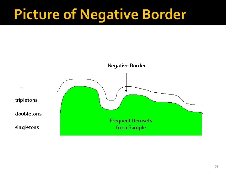
Picture of Negative Border … tripletons doubletons singletons Frequent Itemsets from Sample 45

Toivonen’s Algorithm – (3) �In a second pass, count all candidate frequent itemsets from the first pass, and also count sets in their negative border. �If no itemset from the negative border turns out to be frequent, then the candidates found to be frequent in the whole data are exactly the frequent itemsets. 46

Toivonen’s Algorithm – (4) �What if we find that something in the negative border is actually frequent? �We must start over again with another sample! �Try to choose the support threshold so the probability of failure is low, while the number of itemsets checked on the second pass fits in main-memory. 47

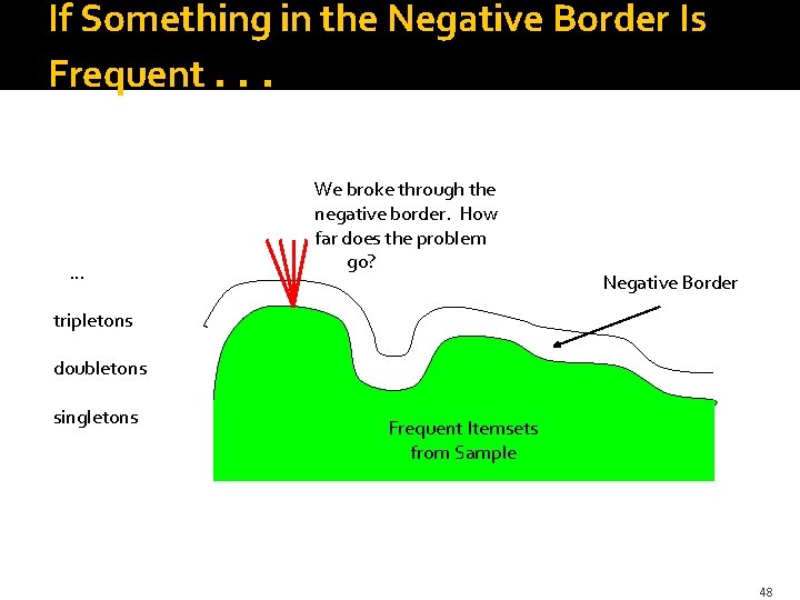
If Something in the Negative Border Is Frequent. . . … We broke through the negative border. How far does the problem go? Negative Border tripletons doubletons singletons Frequent Itemsets from Sample 48

Theorem: �If there is an itemset that is frequent in the whole, but not frequent in the sample, then there is a member of the negative border for the sample that is frequent in the whole. 49

Proof: � Suppose not; i. e. ; 1. There is an itemset S frequent in the whole but not frequent in the sample, and 2. Nothing in the negative border is frequent in the whole. Let T be a smallest subset of S that is not frequent in the sample. � T is frequent in the whole (S is frequent + monotonicity). � T is in the negative border (else not “smallest”). � 50