Association Analysis Association Rule Mining Definition Given a

- Slides: 28

Association Analysis

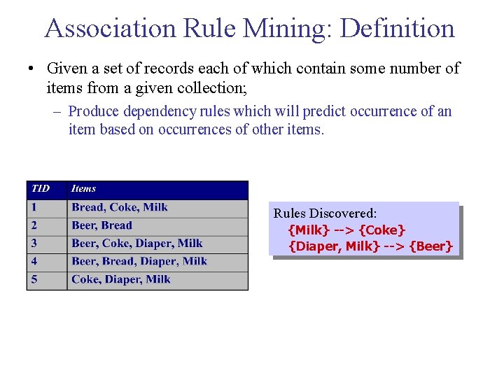
Association Rule Mining: Definition • Given a set of records each of which contain some number of items from a given collection; – Produce dependency rules which will predict occurrence of an item based on occurrences of other items. Rules Discovered: {Milk} --> {Coke} {Diaper, Milk} --> {Beer}

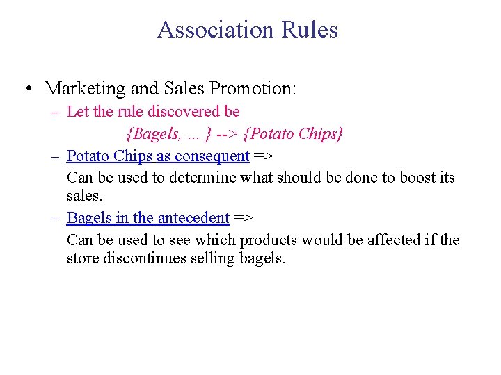
Association Rules • Marketing and Sales Promotion: – Let the rule discovered be {Bagels, … } --> {Potato Chips} – Potato Chips as consequent => Can be used to determine what should be done to boost its sales. – Bagels in the antecedent => Can be used to see which products would be affected if the store discontinues selling bagels.

Two key issues • First, discovering patterns from a large transaction data set can be computationally expensive. • Second, some of the discovered patterns are potentially spurious because they may happen simply by chance.

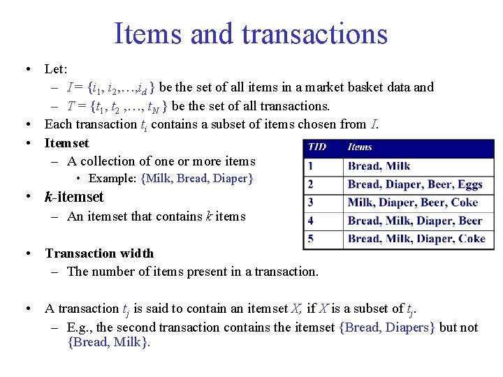
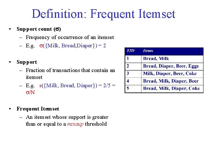
Items and transactions • Let: – I = {i 1, i 2, …, id } be the set of all items in a market basket data and – T = {t 1, t 2 , …, t. N } be the set of all transactions. • Each transaction ti contains a subset of items chosen from I. • Itemset – A collection of one or more items • Example: {Milk, Bread, Diaper} • k-itemset – An itemset that contains k items • Transaction width – The number of items present in a transaction. • A transaction tj is said to contain an itemset X, if X is a subset of tj. – E. g. , the second transaction contains the itemset {Bread, Diapers} but not {Bread, Milk}.

Definition: Frequent Itemset • Support count ( ) – Frequency of occurrence of an itemset – E. g. ({Milk, Bread, Diaper}) = 2 • Support – Fraction of transactions that contain an itemset – E. g. s({Milk, Bread, Diaper}) = 2/5 = /N • Frequent Itemset – An itemset whose support is greater than or equal to a minsup threshold

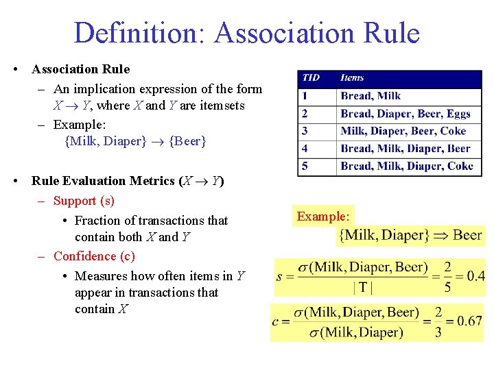
Definition: Association Rule • Association Rule – An implication expression of the form X Y, where X and Y are itemsets – Example: {Milk, Diaper} {Beer} • Rule Evaluation Metrics (X Y) – Support (s) • Fraction of transactions that contain both X and Y – Confidence (c) • Measures how often items in Y appear in transactions that contain X Example:

Why Use Support and Confidence? Support – A rule that has very low support may occur simply by chance. – Support is often used to eliminate uninteresting rules. – Support also has a desirable property that can be exploited for the efficient discovery of association rules. Confidence – Measures the reliability of the inference made by a rule. – For a rule X Y , the higher the confidence, the more likely it is for Y to be present in transactions that contain X. – Confidence provides an estimate of the conditional probability of Y given X.

Association Rule Mining Task • Given a set of transactions T, the goal of association rule mining is to find all rules having – support minsup threshold – confidence minconf threshold • Brute force approach: – List all possible association rules – Compute the support and confidence for each rule – Prune rules that fail the minsup and minconf thresholds Computationally prohibitive!

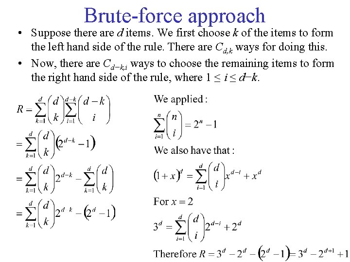
Brute force approach • Suppose there are d items. We first choose k of the items to form the left hand side of the rule. There are Cd, k ways for doing this. • Now, there are Cd−k, i ways to choose the remaining items to form the right hand side of the rule, where 1 ≤ i ≤ d−k.

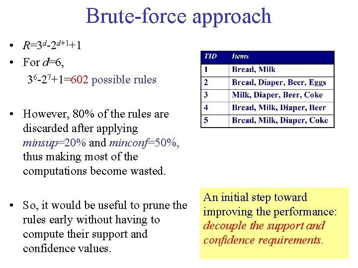
Brute force approach • R=3 d 2 d+1+1 • For d=6, 36 27+1=602 possible rules • However, 80% of the rules are discarded after applying minsup=20% and minconf=50%, thus making most of the computations become wasted. • So, it would be useful to prune the rules early without having to compute their support and confidence values. An initial step toward improving the performance: decouple the support and confidence requirements.

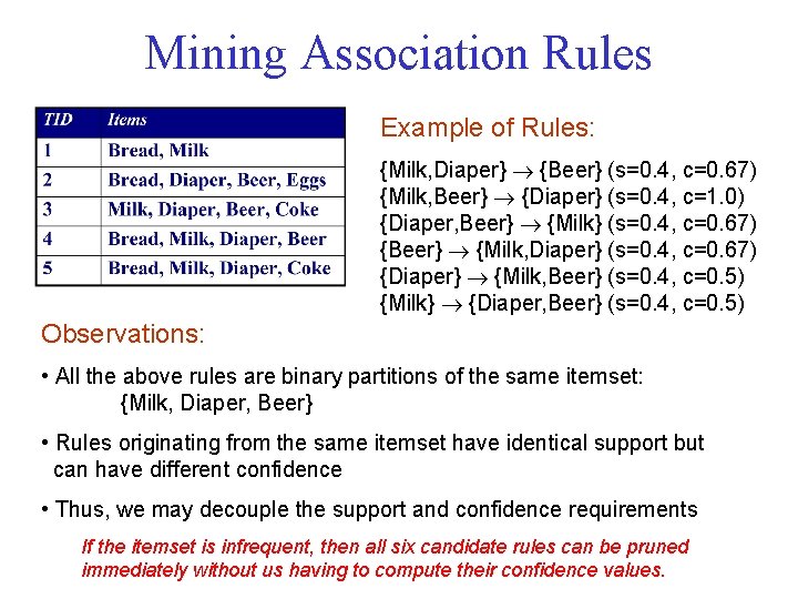
Mining Association Rules Example of Rules: {Milk, Diaper} {Beer} (s=0. 4, c=0. 67) {Milk, Beer} {Diaper} (s=0. 4, c=1. 0) {Diaper, Beer} {Milk} (s=0. 4, c=0. 67) {Beer} {Milk, Diaper} (s=0. 4, c=0. 67) {Diaper} {Milk, Beer} (s=0. 4, c=0. 5) {Milk} {Diaper, Beer} (s=0. 4, c=0. 5) Observations: • All the above rules are binary partitions of the same itemset: {Milk, Diaper, Beer} • Rules originating from the same itemset have identical support but can have different confidence • Thus, we may decouple the support and confidence requirements If the itemset is infrequent, then all six candidate rules can be pruned immediately without us having to compute their confidence values.

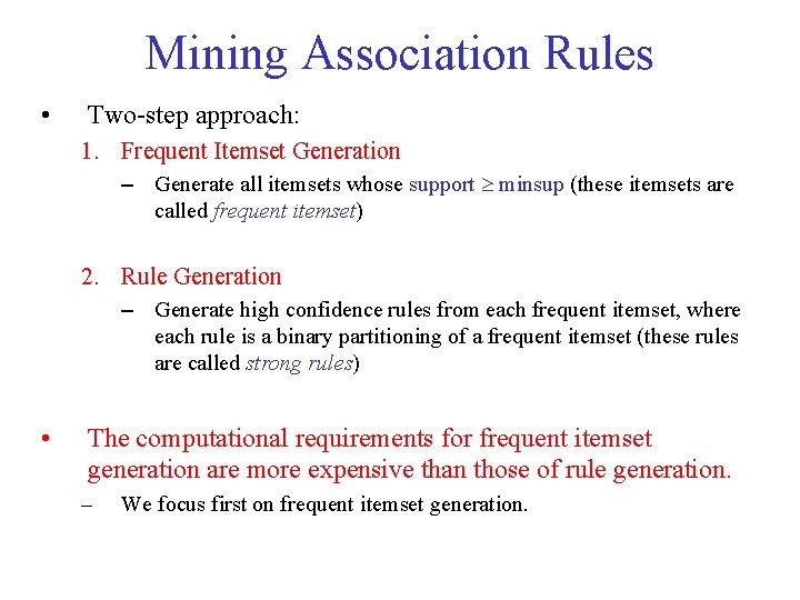
Mining Association Rules • Two step approach: 1. Frequent Itemset Generation – Generate all itemsets whose support minsup (these itemsets are called frequent itemset) 2. Rule Generation – Generate high confidence rules from each frequent itemset, where each rule is a binary partitioning of a frequent itemset (these rules are called strong rules) • The computational requirements for frequent itemset generation are more expensive than those of rule generation. – We focus first on frequent itemset generation.

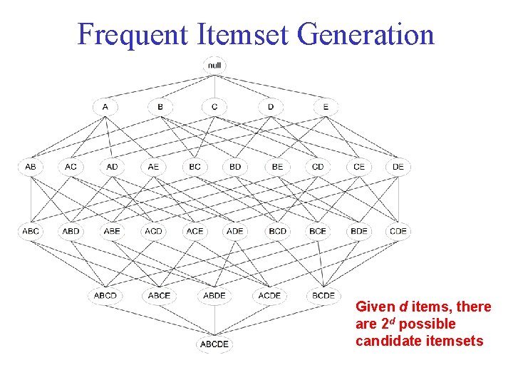
Frequent Itemset Generation Given d items, there are 2 d possible candidate itemsets

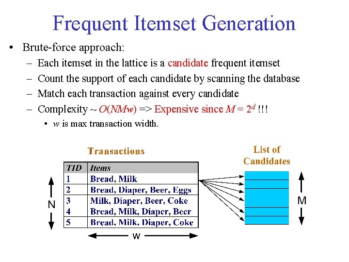
Frequent Itemset Generation • Brute force approach: – – Each itemset in the lattice is a candidate frequent itemset Count the support of each candidate by scanning the database Match each transaction against every candidate Complexity ~ O(NMw) => Expensive since M = 2 d !!! • w is max transaction width.

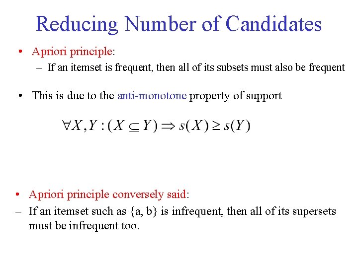
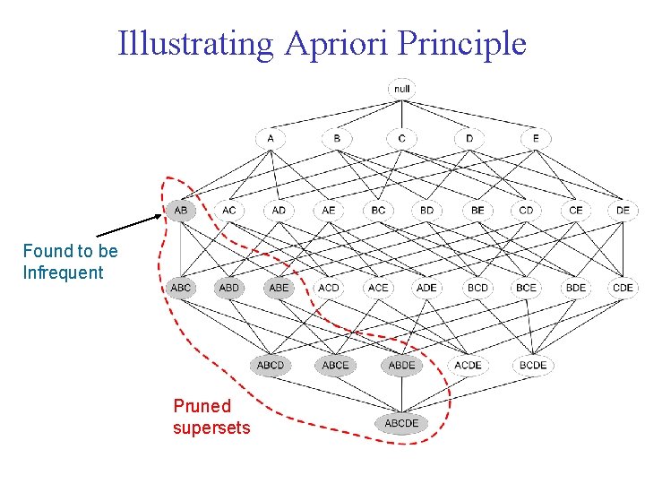
Reducing Number of Candidates • Apriori principle: – If an itemset is frequent, then all of its subsets must also be frequent • This is due to the anti monotone property of support • Apriori principle conversely said: – If an itemset such as {a, b} is infrequent, then all of its supersets must be infrequent too.

Illustrating Apriori Principle Found to be Infrequent Pruned supersets

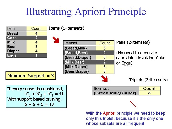
Illustrating Apriori Principle Items (1 -itemsets) Pairs (2 -itemsets) (No need to generate candidates involving Coke or Eggs) Minimum Support = 3 Triplets (3 -itemsets) If every subset is considered, 6 C + 6 C = 41 1 2 3 With support-based pruning, 6 + 1 = 13 With the Apriori principle we need to keep only this triplet, because it’s the only one whose subsets are all frequent.

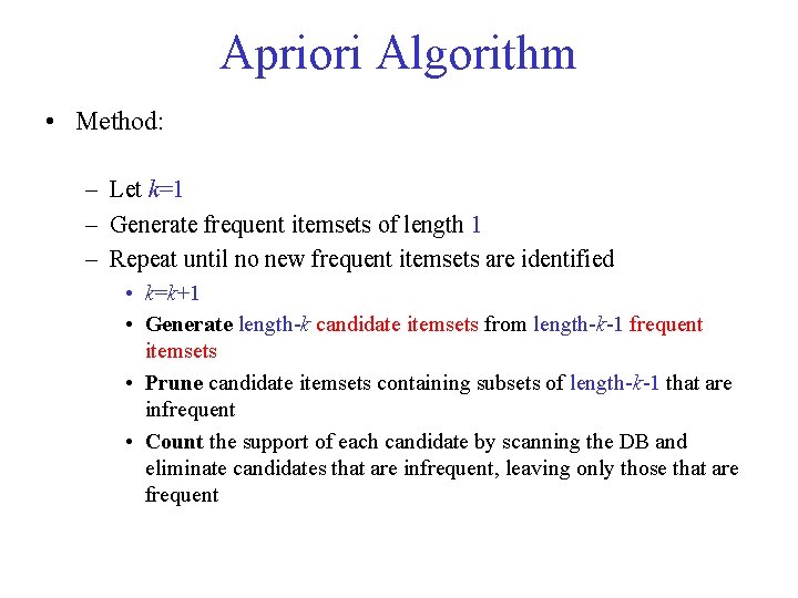
Apriori Algorithm • Method: – Let k=1 – Generate frequent itemsets of length 1 – Repeat until no new frequent itemsets are identified • k=k+1 • Generate length k candidate itemsets from length k 1 frequent itemsets • Prune candidate itemsets containing subsets of length k 1 that are infrequent • Count the support of each candidate by scanning the DB and eliminate candidates that are infrequent, leaving only those that are frequent

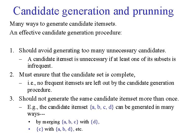
Candidate generation and prunning Many ways to generate candidate itemsets. An effective candidate generation procedure: 1. Should avoid generating too many unnecessary candidates. – A candidate itemset is unnecessary if at least one of its subsets is infrequent. 2. Must ensure that the candidate set is complete, – i. e. , no frequent itemsets are left out by the candidate generation procedure. 3. Should not generate the same candidate itemset more than once. – E. g. , the candidate itemset {a, b, c, d} can be generated in many ways • • by merging {a, b, c} with {d}, {c} with {a, b, d}, etc.

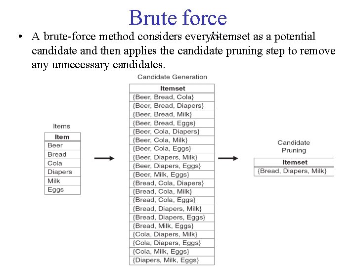
Brute force • A brute force method considers everyk itemset as a potential candidate and then applies the candidate pruning step to remove any unnecessary candidates.

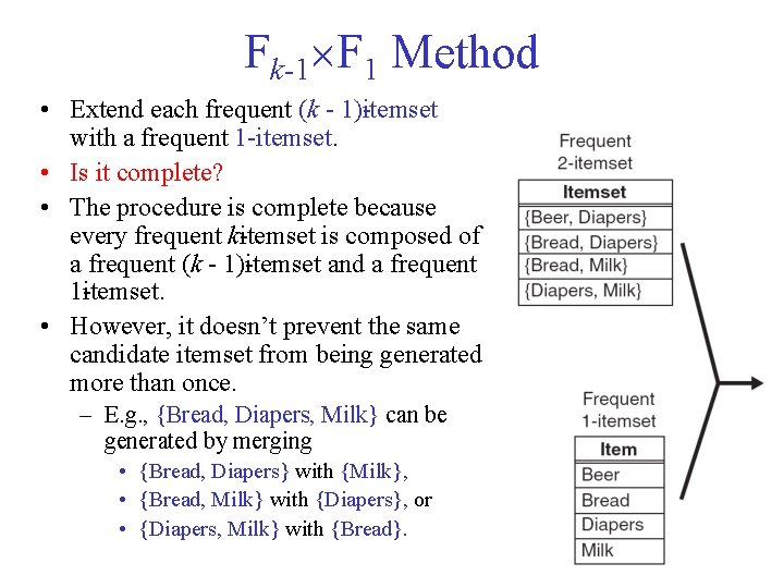
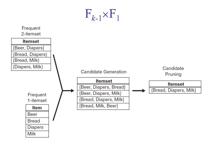
Fk 1 F 1 Method • Extend each frequent (k 1) itemset with a frequent 1 itemset. • Is it complete? • The procedure is complete because every frequent k itemset is composed of a frequent (k 1) itemset and a frequent 1 itemset. • However, it doesn’t prevent the same candidate itemset from being generated more than once. – E. g. , {Bread, Diapers, Milk} can be generated by merging • {Bread, Diapers} with {Milk}, • {Bread, Milk} with {Diapers}, or • {Diapers, Milk} with {Bread}.

Lexicographic Order • Avoid generating duplicate candidates by ensuring that the items in each frequent itemset are kept sorted in their lexicographic order. • Each frequent (k 1) itemset X is then extended with frequent items that are lexicographically larger than the items in X. • For example, the itemset {Bread, Diapers} can be augmented with {Milk} since Milk is lexicographically larger than Bread and Diapers. • However, we don’t augment {Diapers, Milk} with {Bread} nor {Bread, Milk} with {Diapers} because they violate the lexicographic ordering condition. • Is it complete?

Lexicographic Order Completeness • Is it complete? • Yes. Let (i 1, …, ik 1, ik) be a frequent k itemset sorted in lexicographic order. • Since it is frequent, by the Apriori principle, (i 1, …, ik 1) and (ik) are frequent as well. • I. e. (i 1, …, ik 1) Fk 1 and (ik) F 1. • Since, (ik) is lexicographically bigger than i 1, …, ik 1, we have that (i 1, …, ik 1) would be joined with (ik) for giving (i 1, …, ik 1, ik) as a candidate k itemset.

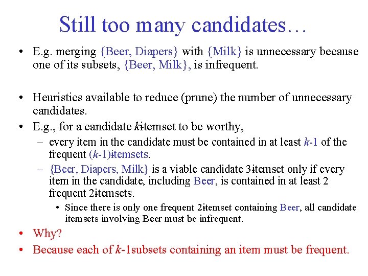
Still too many candidates… • E. g. merging {Beer, Diapers} with {Milk} is unnecessary because one of its subsets, {Beer, Milk}, is infrequent. • Heuristics available to reduce (prune) the number of unnecessary candidates. • E. g. , for a candidate k itemset to be worthy, – every item in the candidate must be contained in at least k 1 of the frequent (k 1) itemsets. – {Beer, Diapers, Milk} is a viable candidate 3 itemset only if every item in the candidate, including Beer, is contained in at least 2 frequent 2 itemsets. • Since there is only one frequent 2 itemset containing Beer, all candidate itemsets involving Beer must be infrequent. • Why? • Because each of k 1 subsets containing an item must be frequent.

Fk 1 F 1

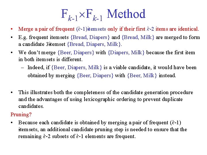
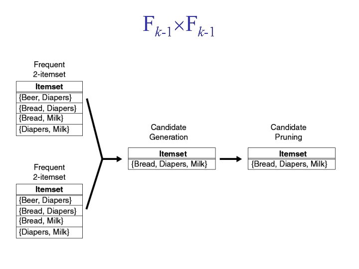
Fk 1 Method • Merge a pair of frequent (k 1) itemsets only if their first k 2 items are identical. • E. g. frequent itemsets {Bread, Diapers} and {Bread, Milk} are merged to form a candidate 3 itemset {Bread, Diapers, Milk}. • We don’t merge {Beer, Diapers} with {Diapers, Milk} because the first item in both itemsets is different. – Indeed, if {Beer, Diapers, Milk} is a viable candidate, it would have been obtained by merging {Beer, Diapers} with {Beer, Milk} instead. • This illustrates both the completeness of the candidate generation procedure and the advantages of using lexicographic ordering to prevent duplicate candidates. Pruning? • Because each candidate is obtained by merging a pair of frequent (k 1) itemsets, an additional candidate pruning step is needed to ensure that the remaining k 2 subsets of k 1 elements are frequent.

Fk 1