Chapter 2 Limits and Continuity 1 2 1

- Slides: 139
Chapter 2 Limits and Continuity 1
2. 1 Rates of Change and Limits 2
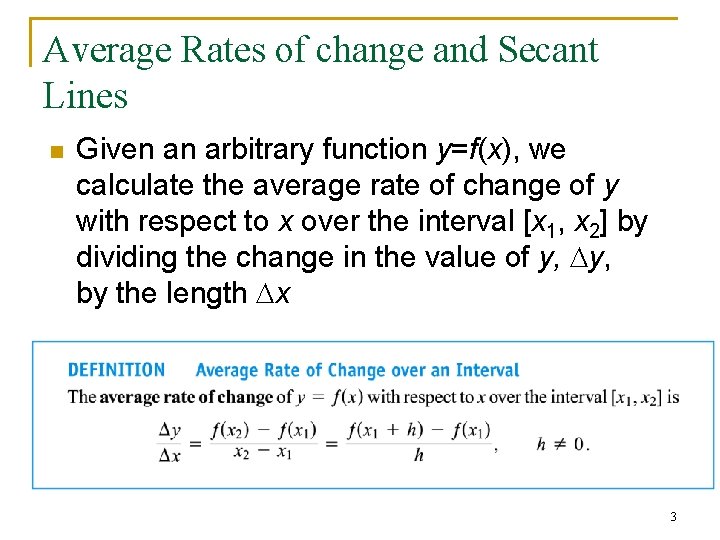
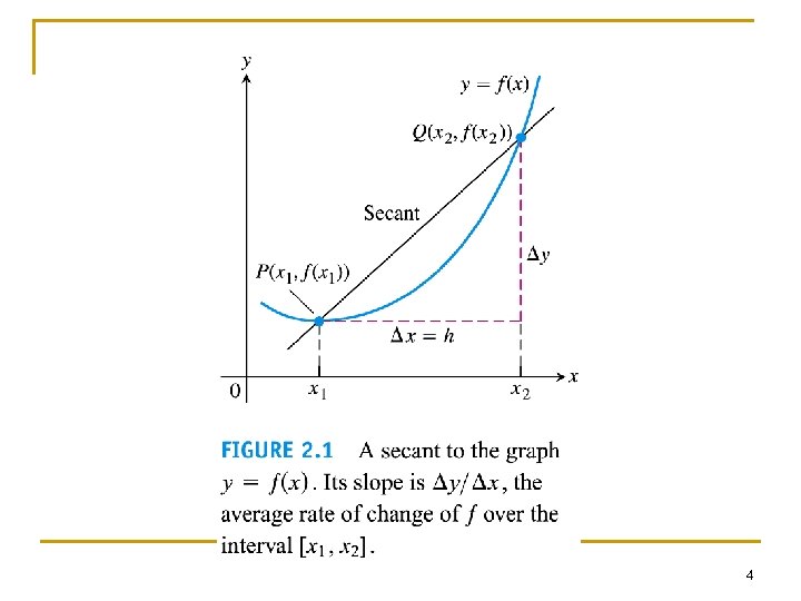
Average Rates of change and Secant Lines n Given an arbitrary function y=f(x), we calculate the average rate of change of y with respect to x over the interval [x 1, x 2] by dividing the change in the value of y, Dy, by the length Dx 3
4
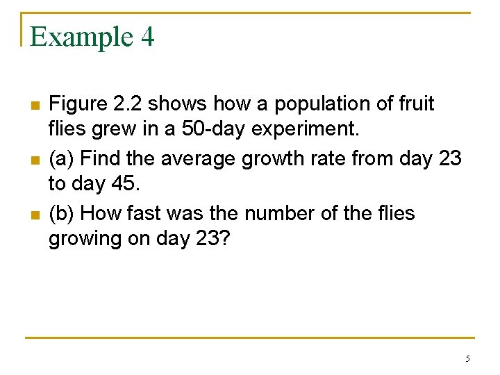
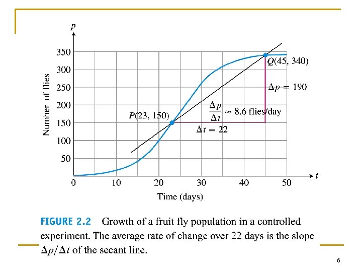
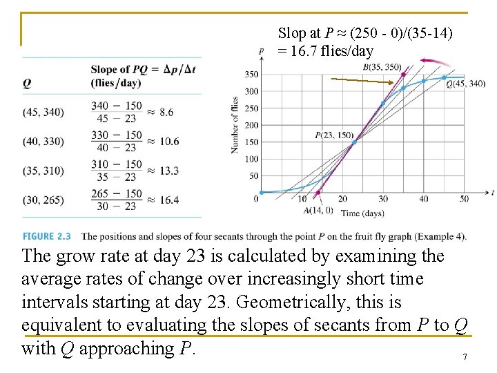
Example 4 n n n Figure 2. 2 shows how a population of fruit flies grew in a 50 -day experiment. (a) Find the average growth rate from day 23 to day 45. (b) How fast was the number of the flies growing on day 23? 5
6
Slop at P ≈ (250 - 0)/(35 -14) = 16. 7 flies/day The grow rate at day 23 is calculated by examining the average rates of change over increasingly short time intervals starting at day 23. Geometrically, this is equivalent to evaluating the slopes of secants from P to Q with Q approaching P. 7
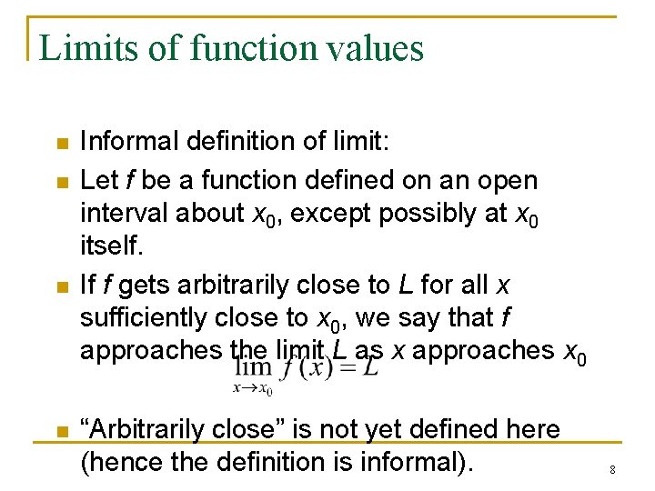
Limits of function values n n Informal definition of limit: Let f be a function defined on an open interval about x 0, except possibly at x 0 itself. If f gets arbitrarily close to L for all x sufficiently close to x 0, we say that f approaches the limit L as x approaches x 0 “Arbitrarily close” is not yet defined here (hence the definition is informal). 8
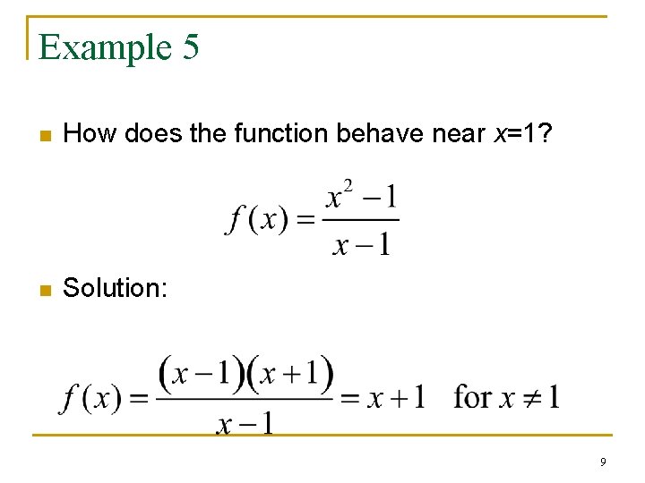
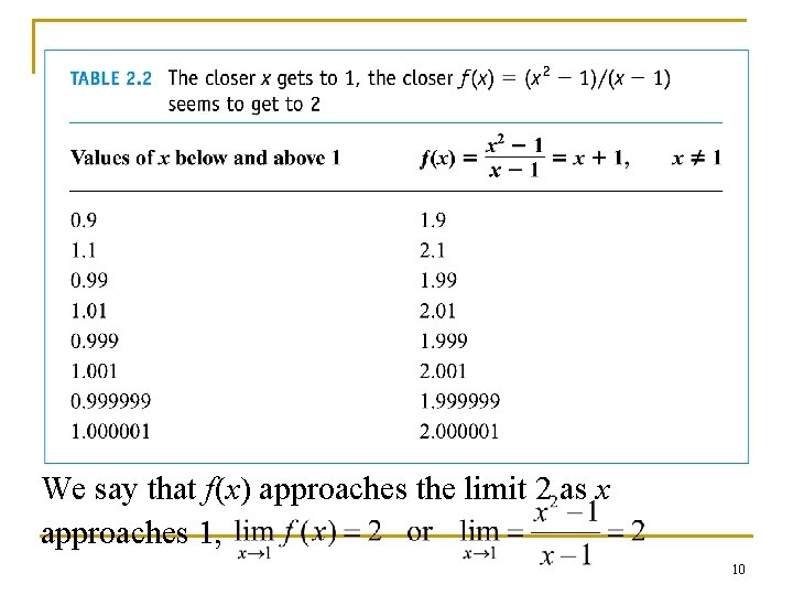
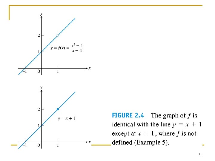
Example 5 n How does the function behave near x=1? n Solution: 9
We say that f(x) approaches the limit 2 as x approaches 1, 10
11
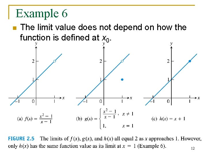
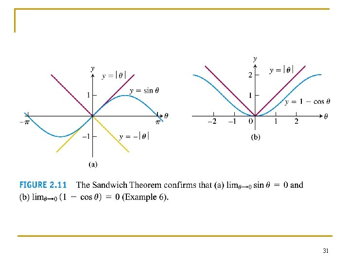
Example 6 n The limit value does not depend on how the function is defined at x 0. 12
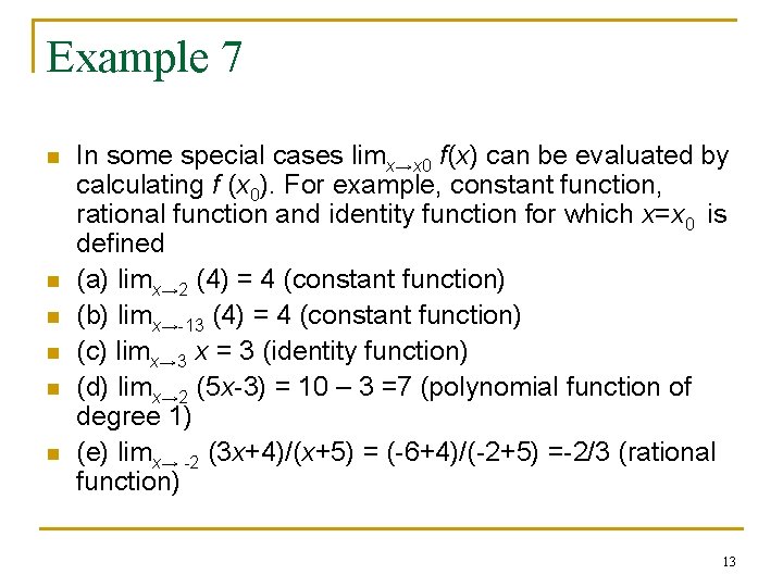
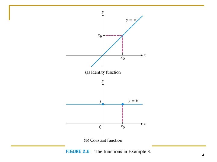
Example 7 n n n In some special cases limx→x 0 f(x) can be evaluated by calculating f (x 0). For example, constant function, rational function and identity function for which x=x 0 is defined (a) limx→ 2 (4) = 4 (constant function) (b) limx→-13 (4) = 4 (constant function) (c) limx→ 3 x = 3 (identity function) (d) limx→ 2 (5 x-3) = 10 – 3 =7 (polynomial function of degree 1) (e) limx→ -2 (3 x+4)/(x+5) = (-6+4)/(-2+5) =-2/3 (rational function) 13
14
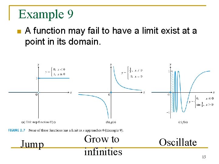
Example 9 n A function may fail to have a limit exist at a point in its domain. Jump Grow to infinities Oscillate 15
2. 2 Calculating limits using the limits laws 16
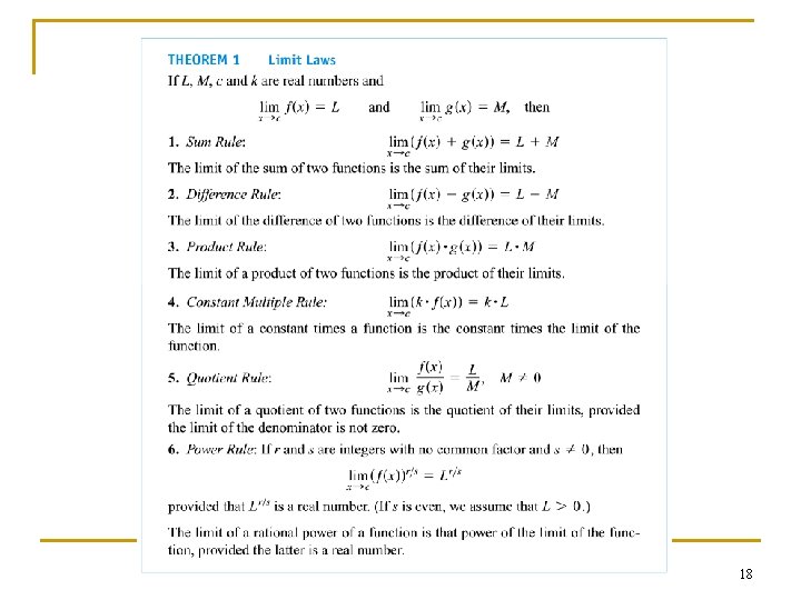
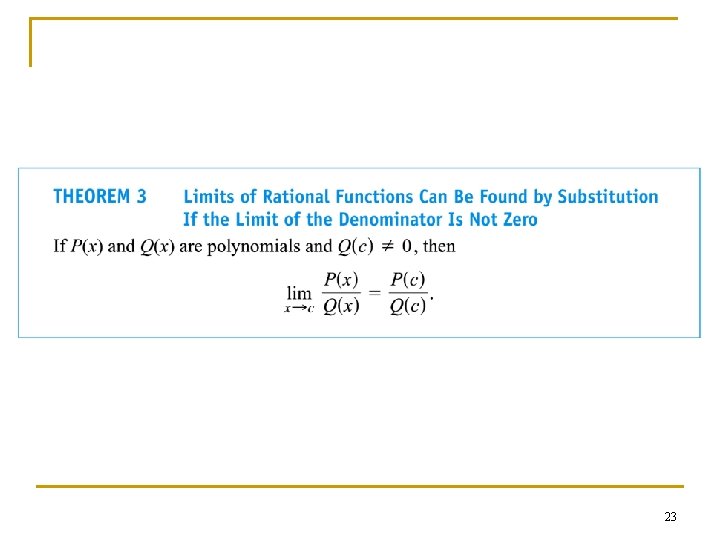
The limit laws n Theorem 1 tells how to calculate limits of functions that are arithmetic combinations of functions whose limit are already known. 17
18
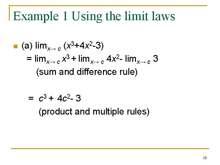
Example 1 Using the limit laws n (a) limx→ c (x 3+4 x 2 -3) = limx→ c x 3 + limx→ c 4 x 2 - limx→ c 3 (sum and difference rule) = c 3 + 4 c 2 - 3 (product and multiple rules) 19
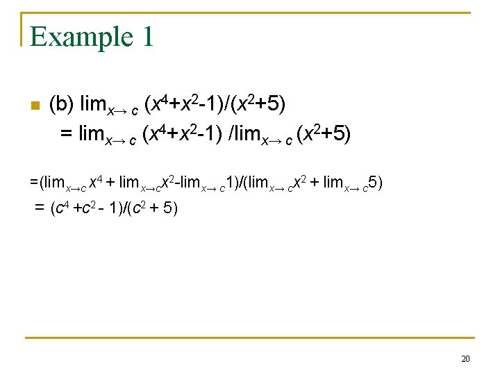
Example 1 n (b) limx→ c (x 4+x 2 -1)/(x 2+5) = limx→ c (x 4+x 2 -1) /limx→ c (x 2+5) =(limx→c x 4 + limx→cx 2 -limx→ c 1)/(limx→ cx 2 + limx→ c 5) = (c 4 +c 2 - 1)/(c 2 + 5) 20
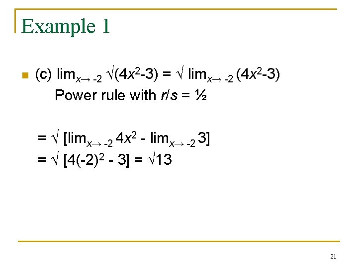
Example 1 n (c) limx→ -2 (4 x 2 -3) = limx→ -2 (4 x 2 -3) Power rule with r/s = ½ = [limx→ -2 4 x 2 - limx→ -2 3] = [4(-2)2 - 3] = 13 21
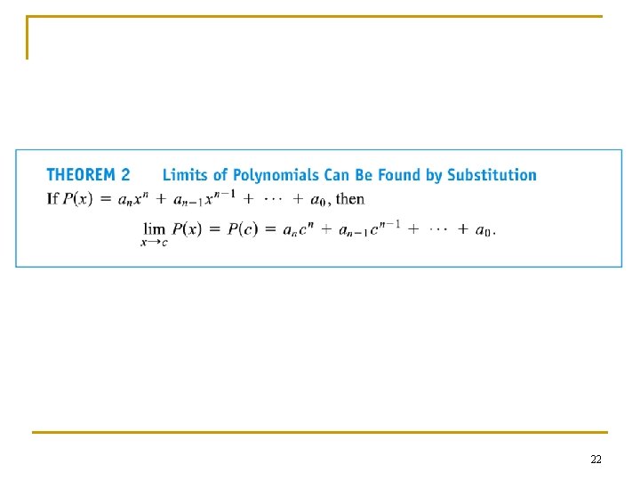
22
23
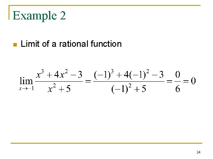
Example 2 n Limit of a rational function 24
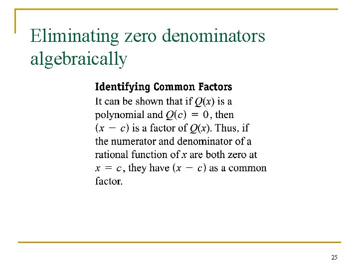
Eliminating zero denominators algebraically 25
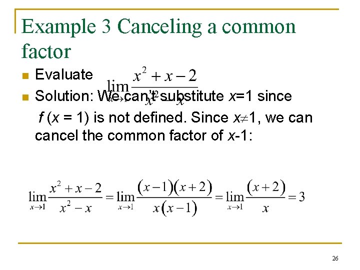
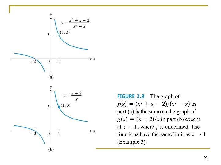
Example 3 Canceling a common factor n n Evaluate Solution: We can’t substitute x=1 since f (x = 1) is not defined. Since x 1, we cancel the common factor of x-1: 26
27
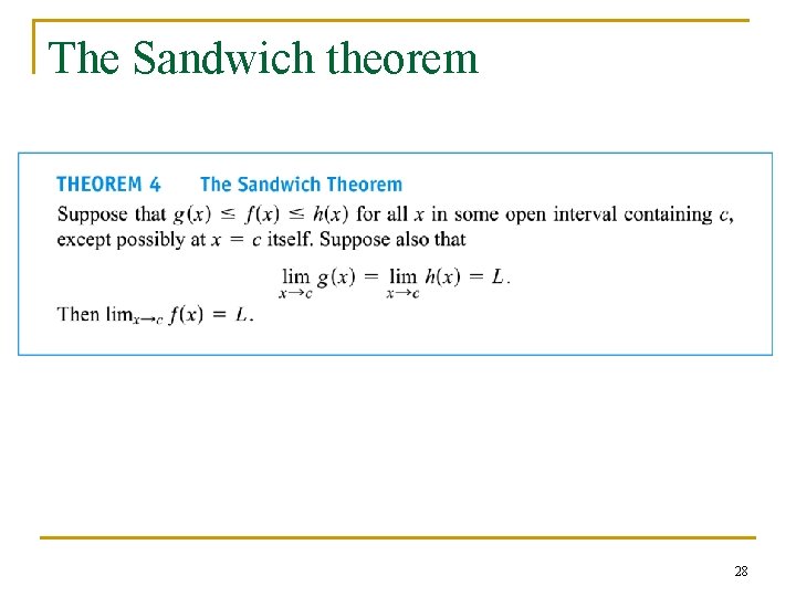
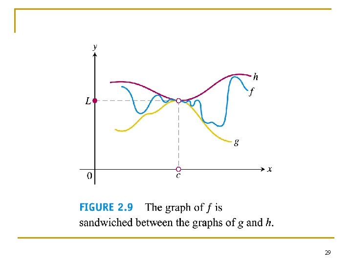
The Sandwich theorem 28
29
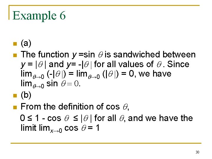
Example 6 n n (a) The function y =sin q is sandwiched between y = |q | and y= -|q | for all values of q. Since limq→ 0 (-|q |) = limq→ 0 (|q |) = 0, we have limq→ 0 sin q = 0. (b) From the definition of cos q, 0 ≤ 1 - cos q ≤ |q | for all q, and we have the limit limx→ 0 cos q = 1 30
31
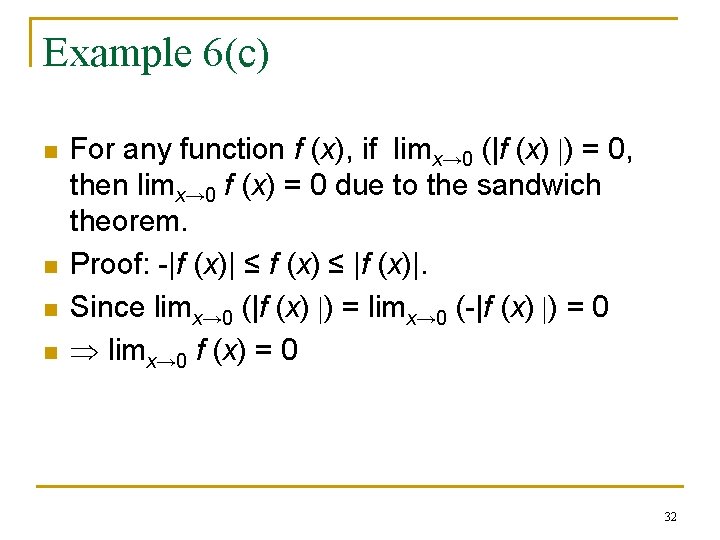
Example 6(c) n n For any function f (x), if limx→ 0 (|f (x) |) = 0, then limx→ 0 f (x) = 0 due to the sandwich theorem. Proof: -|f (x)| ≤ f (x) ≤ |f (x)|. Since limx→ 0 (|f (x) |) = limx→ 0 (-|f (x) |) = 0 limx→ 0 f (x) = 0 32
2. 3 The Precise Definition of a Limit 33
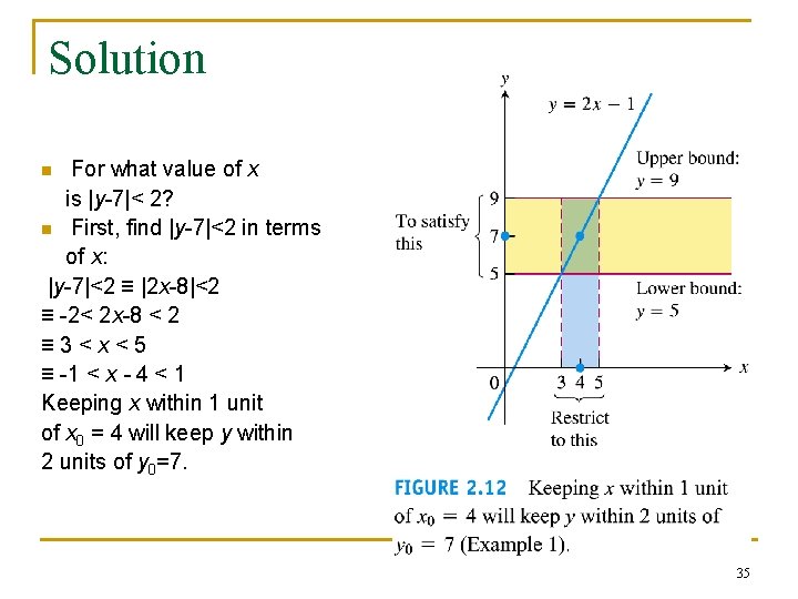
Example 1 A linear function n Consider the linear function y = 2 x – 1 near x 0 = 4. Intuitively it is close to 7 when x is close to 4, so limx 0 (2 x-1)=7. How close does x have to be so that y = 2 x -1 differs from 7 by less than 2 units? 34
Solution For what value of x is |y-7|< 2? n First, find |y-7|<2 in terms of x: |y-7|<2 ≡ |2 x-8|<2 ≡ -2< 2 x-8 < 2 ≡ 3<x<5 ≡ -1 < x - 4 < 1 Keeping x within 1 unit of x 0 = 4 will keep y within 2 units of y 0=7. n 35
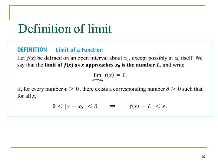
Definition of limit 36
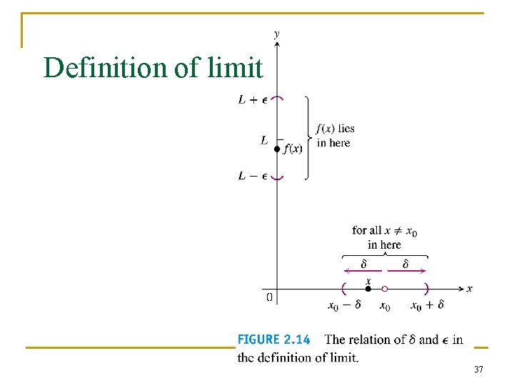
Definition of limit 37
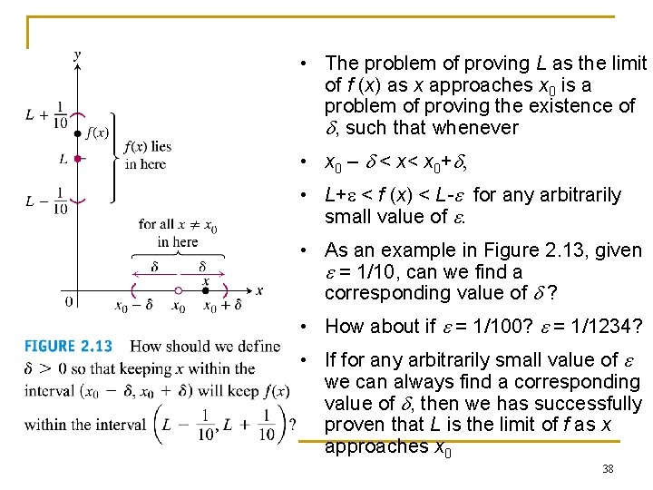
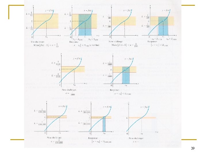
• The problem of proving L as the limit of f (x) as x approaches x 0 is a problem of proving the existence of d, such that whenever • x 0 – d < x< x 0+d, • L+e < f (x) < L-e for any arbitrarily small value of e. • As an example in Figure 2. 13, given e = 1/10, can we find a corresponding value of d ? • How about if e = 1/100? e = 1/1234? • If for any arbitrarily small value of e we can always find a corresponding value of d, then we has successfully proven that L is the limit of f as x approaches x 0 38
39
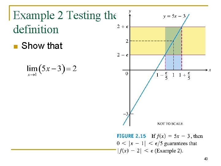
Example 2 Testing the definition n Show that 40
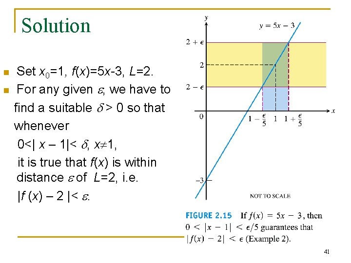
Solution n n Set x 0=1, f(x)=5 x-3, L=2. For any given e, we have to find a suitable d > 0 so that whenever 0<| x – 1|< d, x 1, it is true that f(x) is within distance e of L=2, i. e. |f (x) – 2 |< e. 41
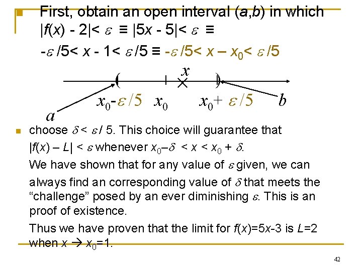
n First, obtain an open interval (a, b) in which |f(x) - 2|< e ≡ |5 x - 5|< e ≡ -e /5< x - 1< e /5 ≡ -e /5< x – x 0< e /5 a n ( x 0 -e /5 x 0 x ) x 0+ e /5 b choose d < e / 5. This choice will guarantee that |f(x) – L| < e whenever x 0–d < x 0 + d. We have shown that for any value of e given, we can always find an corresponding value of d that meets the “challenge” posed by an ever diminishing e. This is an proof of existence. Thus we have proven that the limit for f(x)=5 x-3 is L=2 when x x 0=1. 42
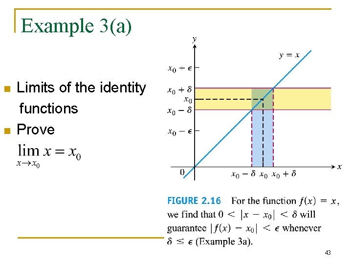
Example 3(a) n n Limits of the identity functions Prove 43
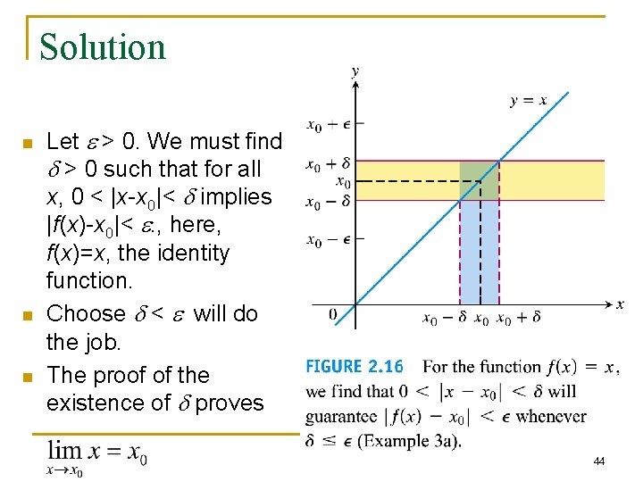
Solution n Let e > 0. We must find d > 0 such that for all x, 0 < |x-x 0|< d implies |f(x)-x 0|< e. , here, f(x)=x, the identity function. Choose d < e will do the job. The proof of the existence of d proves 44
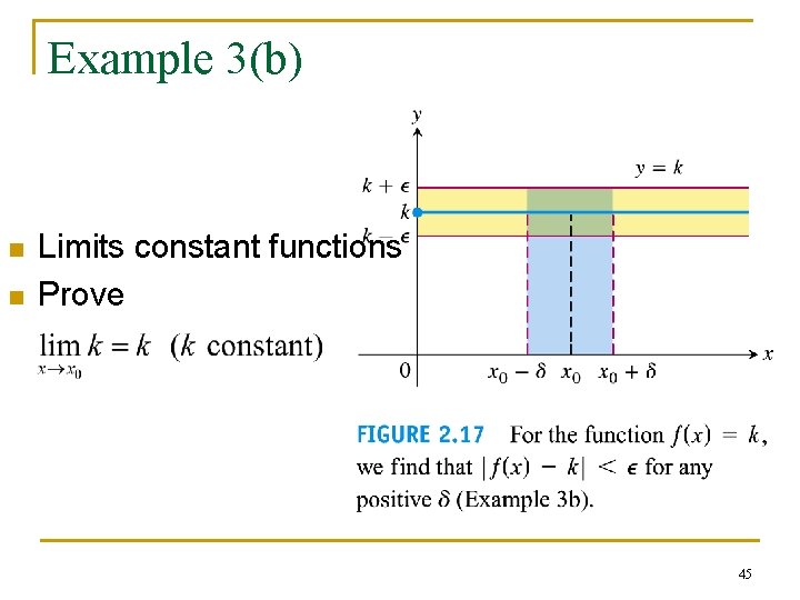
Example 3(b) n n Limits constant functions Prove 45
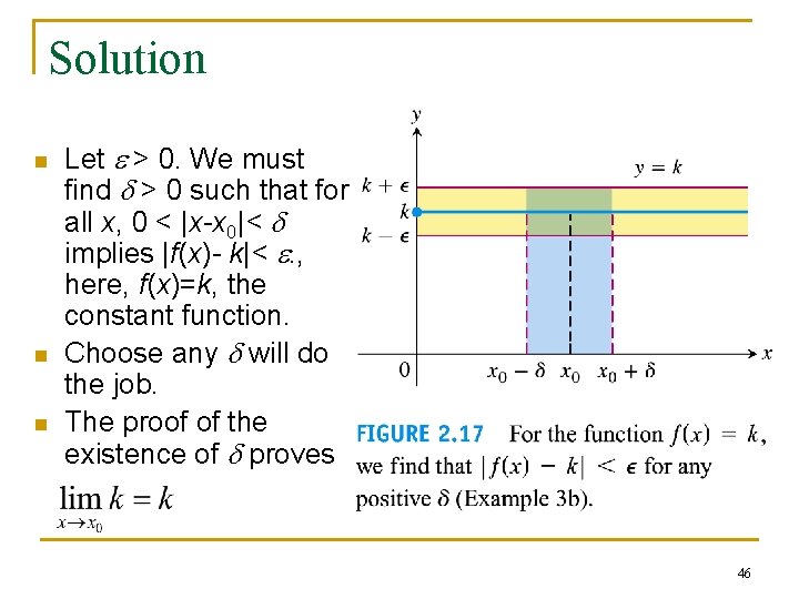
Solution n Let e > 0. We must find d > 0 such that for all x, 0 < |x-x 0|< d implies |f(x)- k|< e. , here, f(x)=k, the constant function. Choose any d will do the job. The proof of the existence of d proves 46
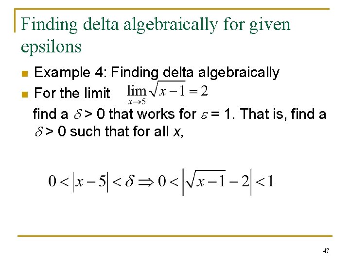
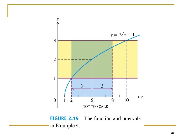
Finding delta algebraically for given epsilons n n Example 4: Finding delta algebraically For the limit find a d > 0 that works for e = 1. That is, find a d > 0 such that for all x, 47
48
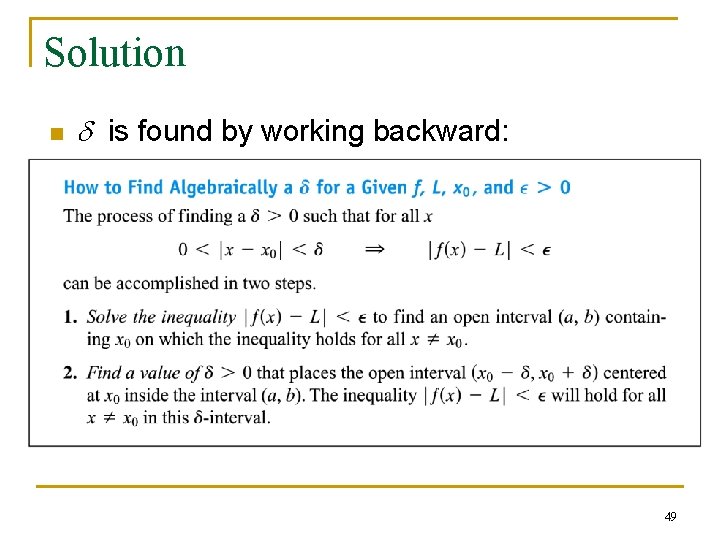
Solution n d is found by working backward: 49
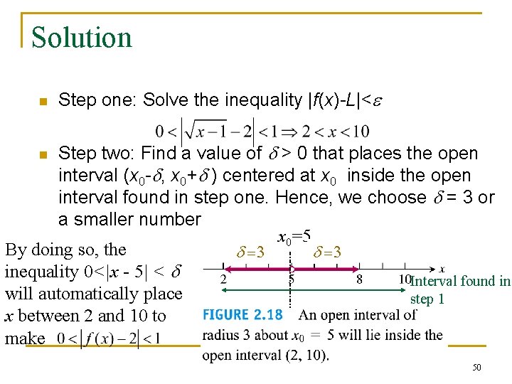
Solution n Step one: Solve the inequality |f(x)-L|<e Step two: Find a value of d > 0 that places the open interval (x 0 -d, x 0+d ) centered at x 0 inside the open interval found in step one. Hence, we choose d = 3 or a smaller number x 0=5 By doing so, the d =3 inequality 0<|x - 5| < d Interval found in will automatically place step 1 x between 2 and 10 to make n 50
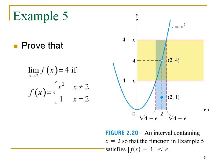
Example 5 n Prove that 51
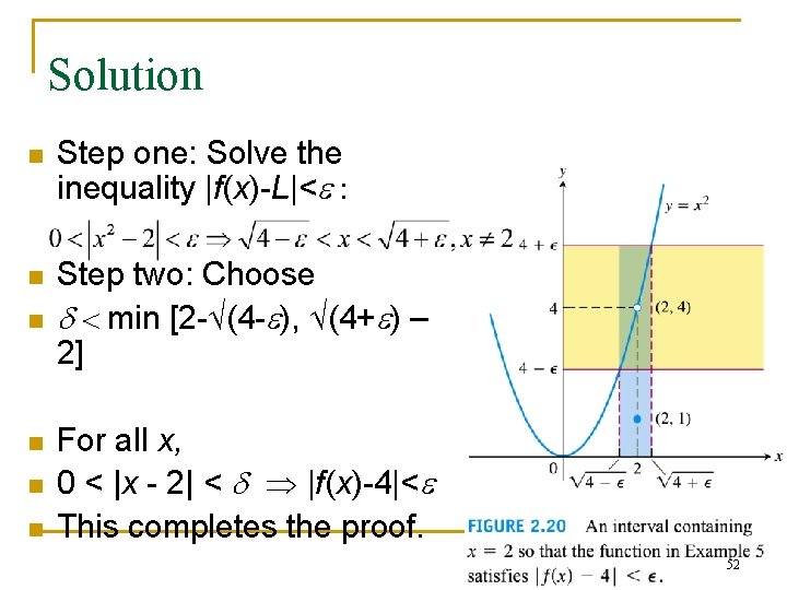
Solution n Step one: Solve the inequality |f(x)-L|<e : n Step two: Choose d < min [2 - (4 -e), (4+e) – 2] n n For all x, 0 < |x - 2| < d |f(x)-4|<e This completes the proof. 52
2. 4 One-Sided Limits and Limits at Infinity 53
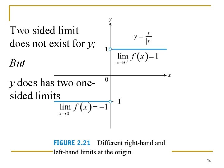
Two sided limit does not exist for y; But y does has two onesided limits 54
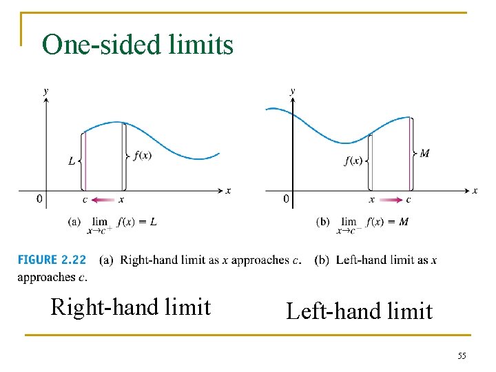
One-sided limits Right-hand limit Left-hand limit 55
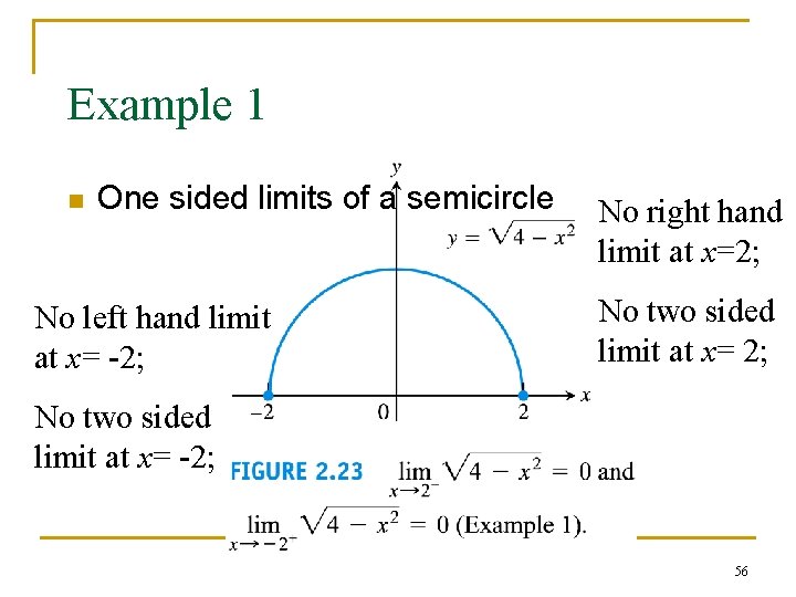
Example 1 n One sided limits of a semicircle No left hand limit at x= -2; No right hand limit at x=2; No two sided limit at x= 2; No two sided limit at x= -2; 56
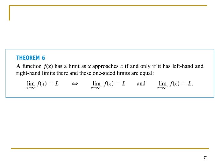
57
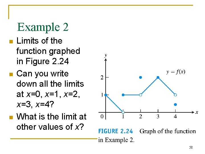
Example 2 n n n Limits of the function graphed in Figure 2. 24 Can you write down all the limits at x=0, x=1, x=2, x=3, x=4? What is the limit at other values of x? 58
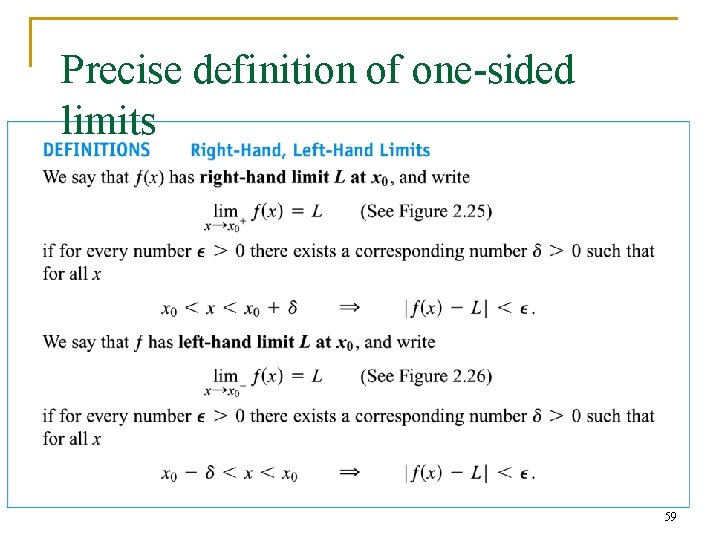
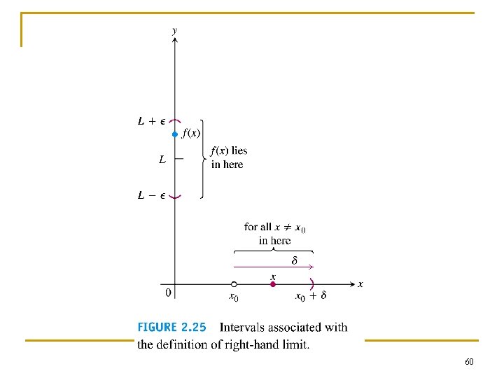
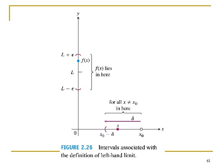
Precise definition of one-sided limits 59
60
61
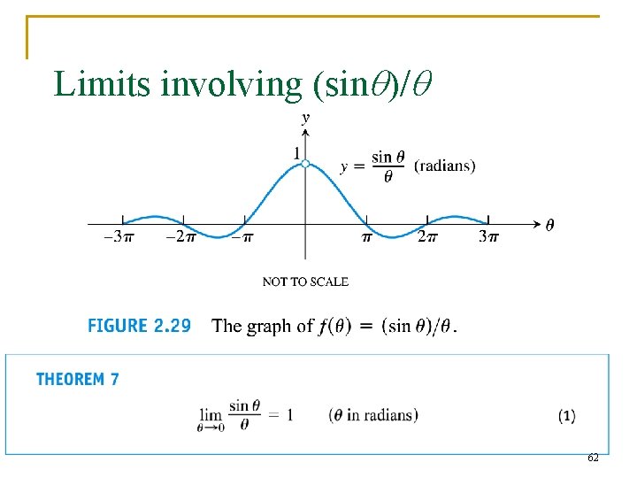
Limits involving (sinq)/q 62
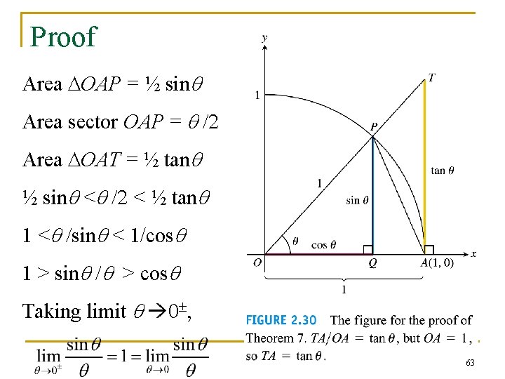
Proof Area DOAP = ½ sinq Area sector OAP = q /2 Area DOAT = ½ tanq ½ sinq <q /2 < ½ tanq 1 <q /sinq < 1/cosq 1 > sinq /q > cosq Taking limit q 0 , 63
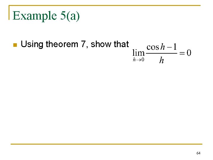
Example 5(a) n Using theorem 7, show that 64
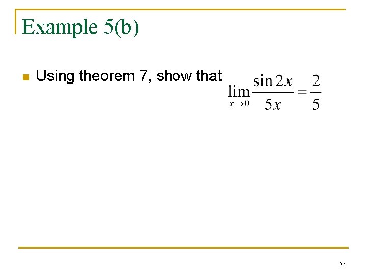
Example 5(b) n Using theorem 7, show that 65
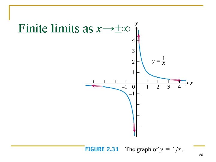
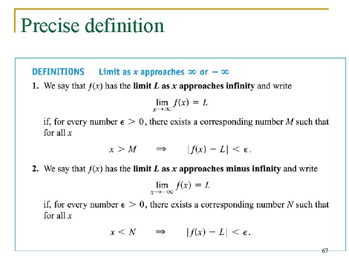
Finite limits as x→ ∞ 66
Precise definition 67
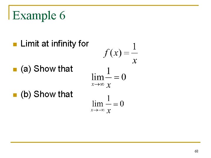
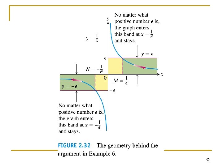
Example 6 n Limit at infinity for n (a) Show that n (b) Show that 68
69
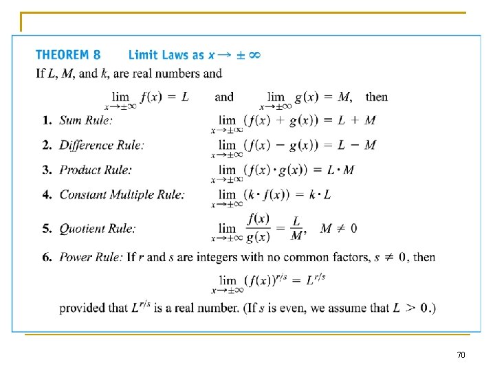
70
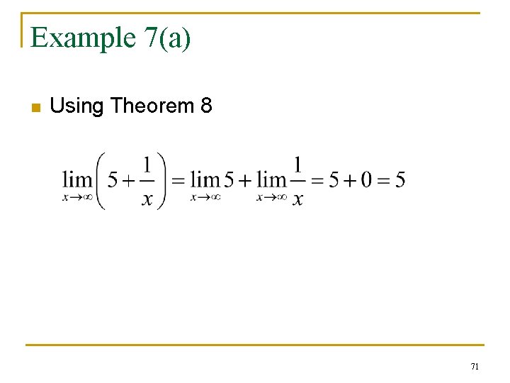
Example 7(a) n Using Theorem 8 71
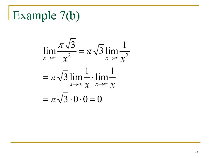
Example 7(b) 72
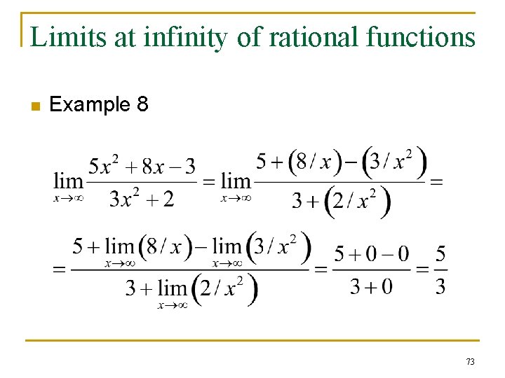
Limits at infinity of rational functions n Example 8 73
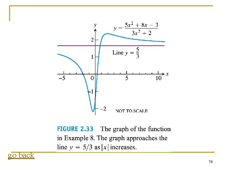
go back 74
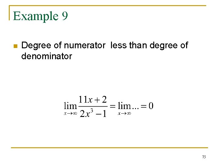
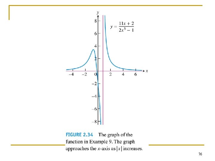
Example 9 n Degree of numerator less than degree of denominator 75
76
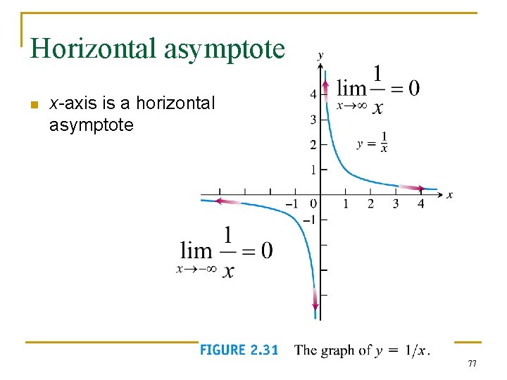
Horizontal asymptote n x-axis is a horizontal asymptote 77
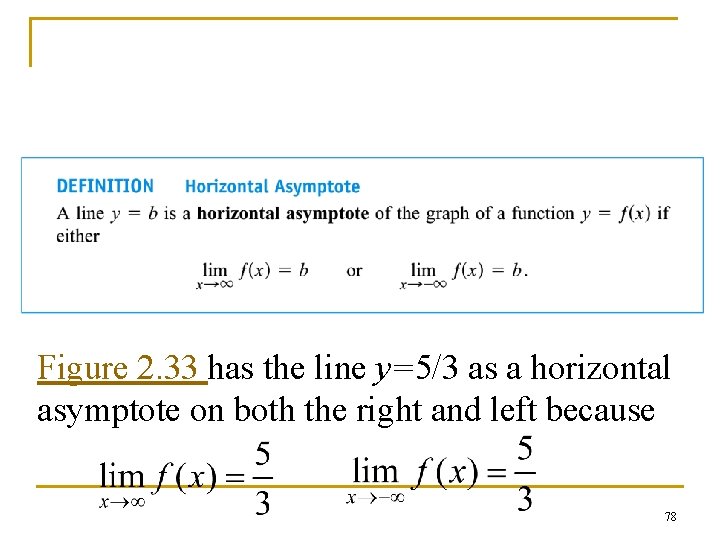
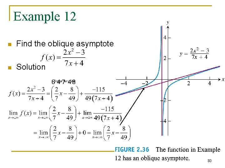
Figure 2. 33 has the line y=5/3 as a horizontal asymptote on both the right and left because 78
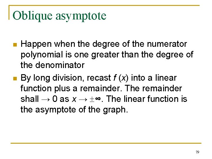
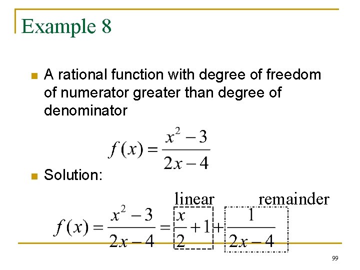
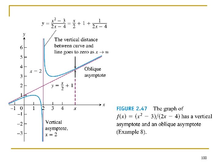
Oblique asymptote n n Happen when the degree of the numerator polynomial is one greater than the degree of the denominator By long division, recast f (x) into a linear function plus a remainder. The remainder shall → 0 as x → ∞. The linear function is the asymptote of the graph. 79
Example 12 n Find the oblique asymptote for n Solution 80
2. 5 Infinite Limits and Vertical Asymptotes 81
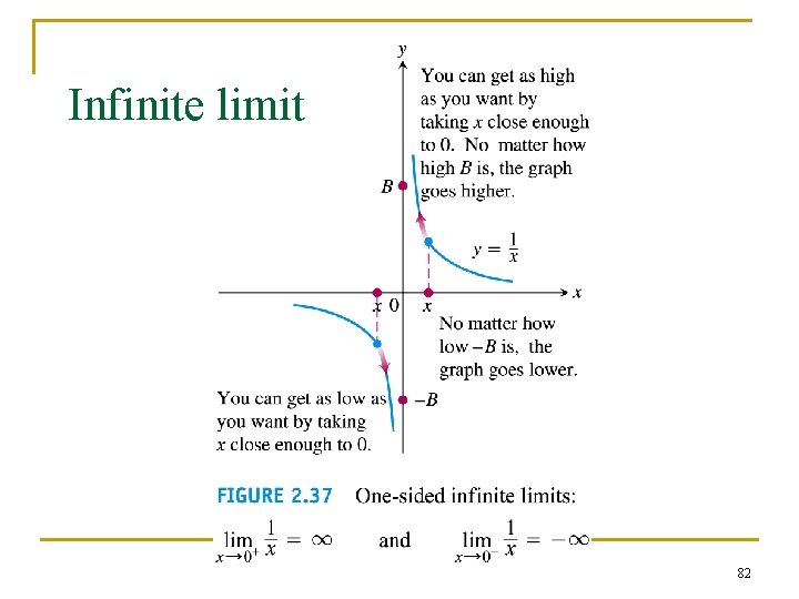
Infinite limit 82
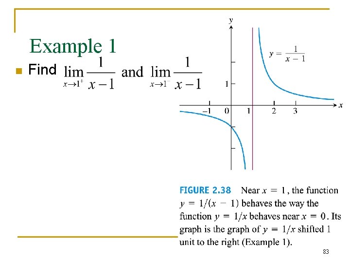
Example 1 n Find 83
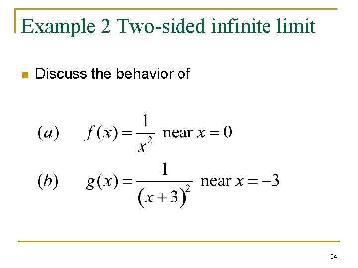
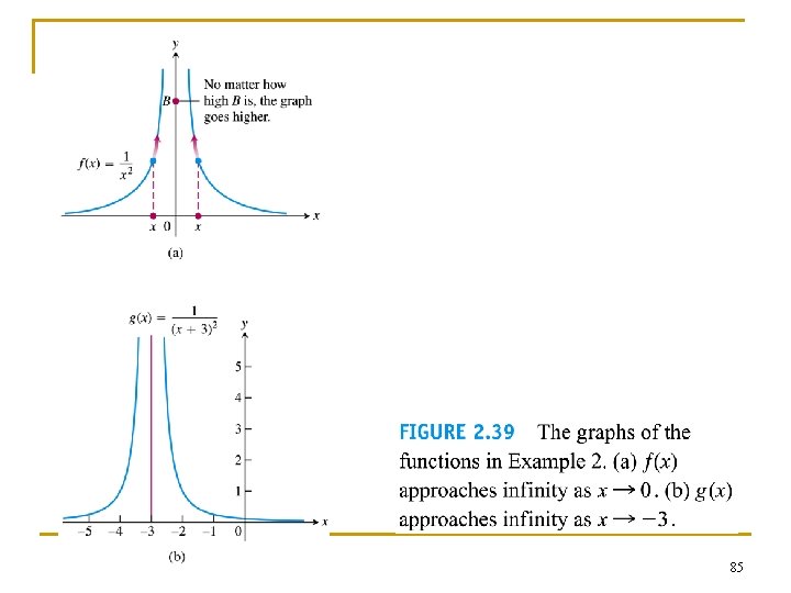
Example 2 Two-sided infinite limit n Discuss the behavior of 84
85
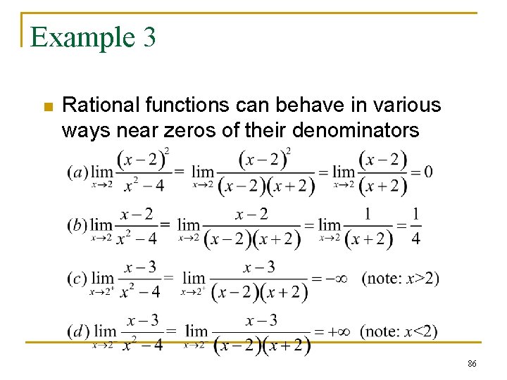
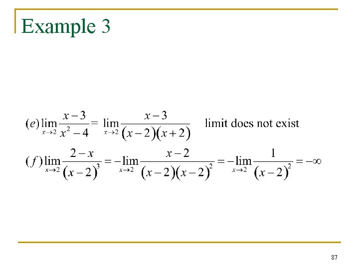
Example 3 n Rational functions can behave in various ways near zeros of their denominators 86
Example 3 87
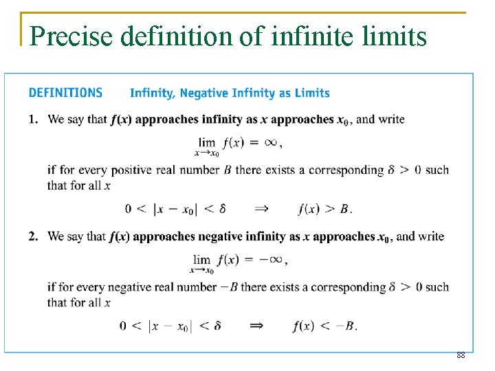
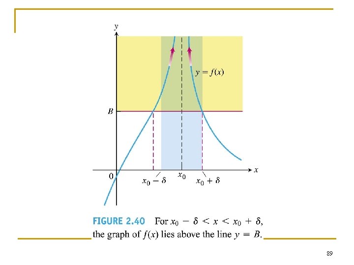
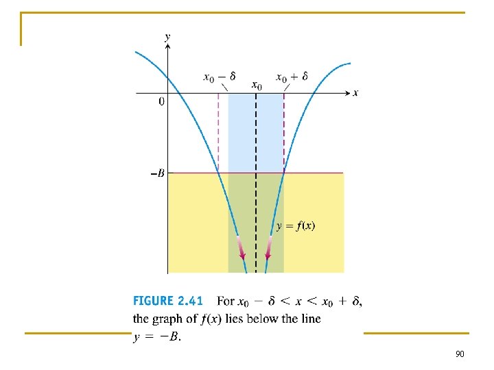
Precise definition of infinite limits 88
89
90
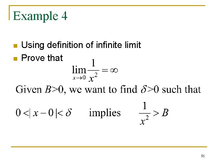
Example 4 n n Using definition of infinite limit Prove that 91
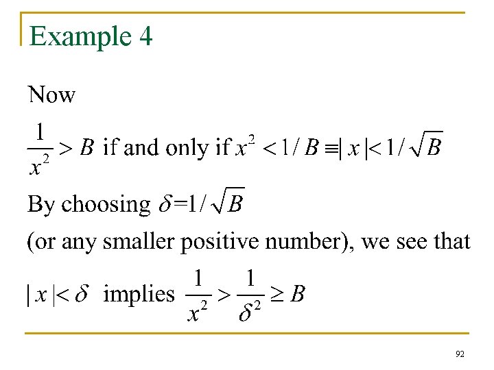
Example 4 92
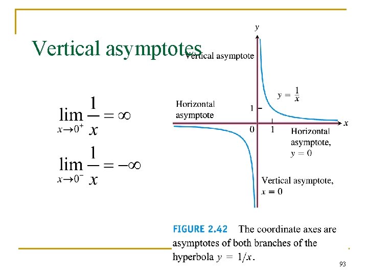
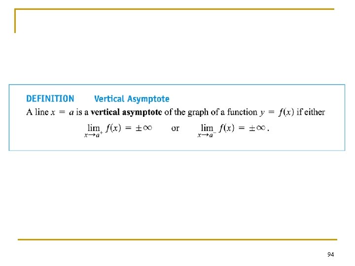
Vertical asymptotes 93
94
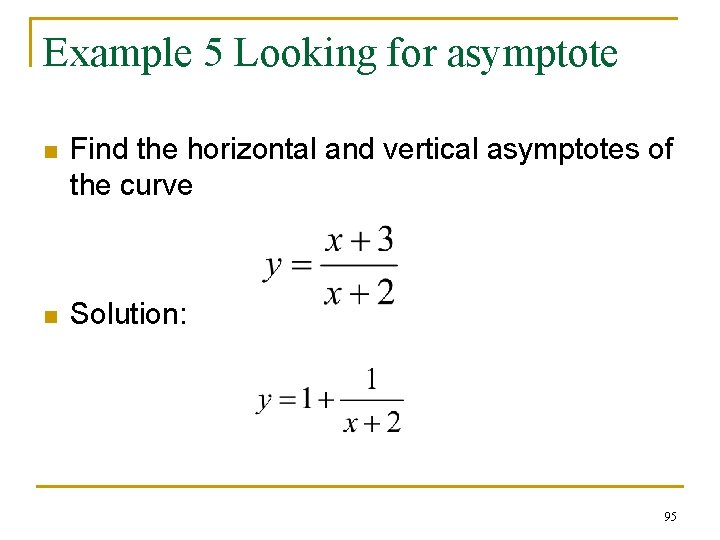
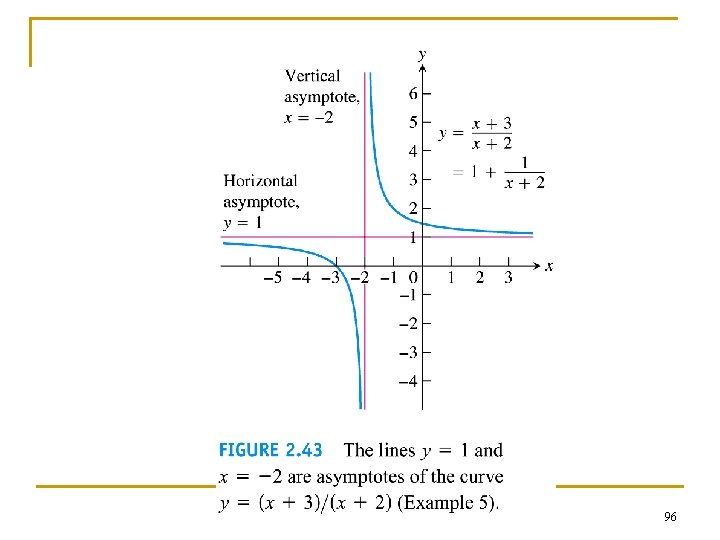
Example 5 Looking for asymptote n Find the horizontal and vertical asymptotes of the curve n Solution: 95
96
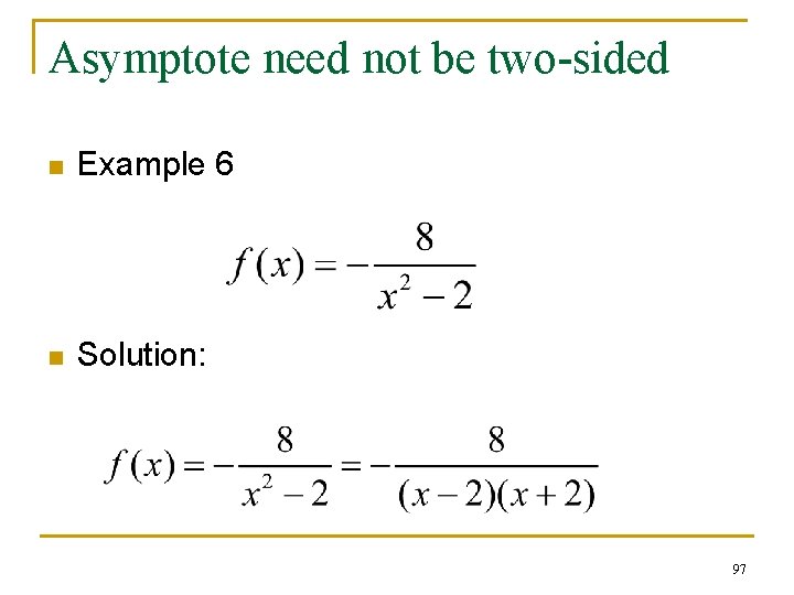
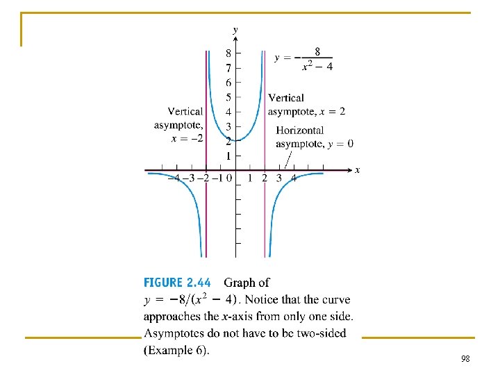
Asymptote need not be two-sided n Example 6 n Solution: 97
98
Example 8 n A rational function with degree of freedom of numerator greater than degree of denominator n Solution: linear remainder 99
100
2. 6 Continuity 101
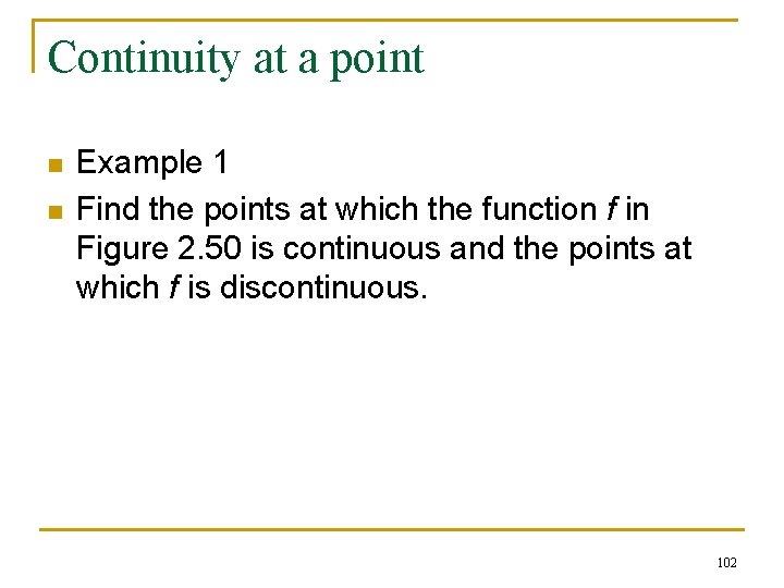
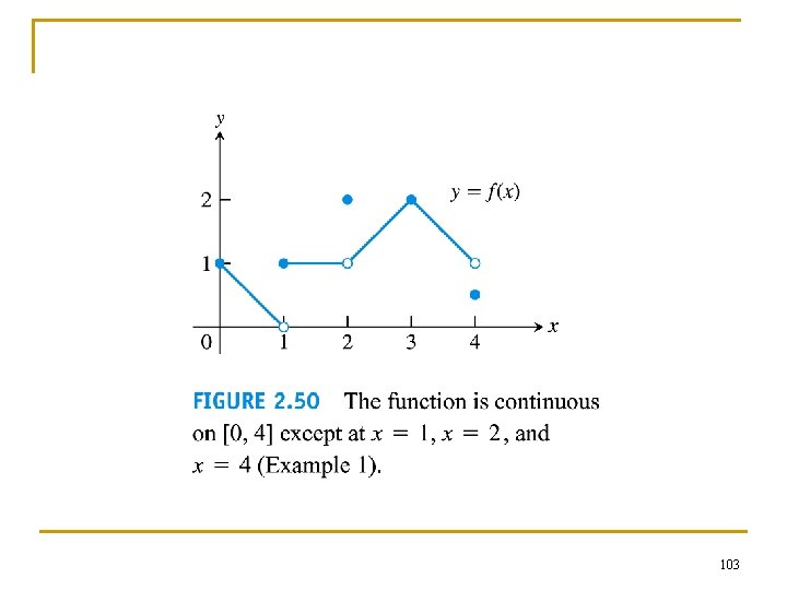
Continuity at a point n n Example 1 Find the points at which the function f in Figure 2. 50 is continuous and the points at which f is discontinuous. 102
103
n n f continuous: At x = 0 At x = 3 At 0 < c < 4, c 1, 2 n n n f discontinuous: At x = 1 At x = 2 At x = 4 0 > c, c > 4 Why? 104
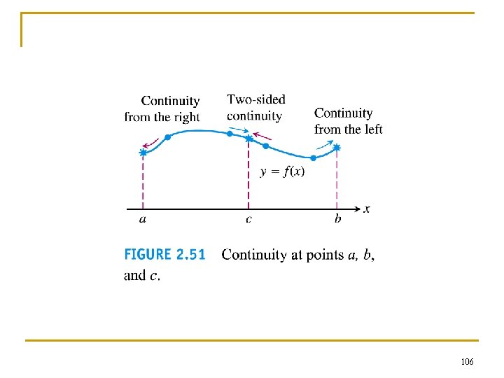
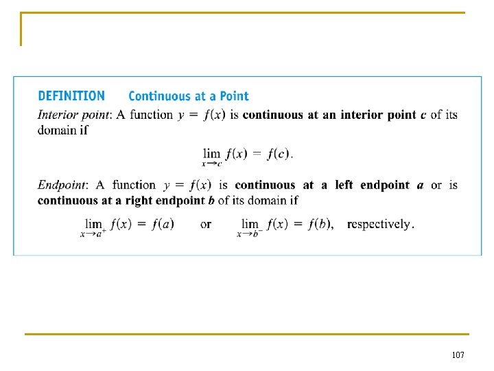
n n n To define the continuity at a point in a function’s domain, we need to define continuity at an interior point define continuity at an endpoint 105
106
107
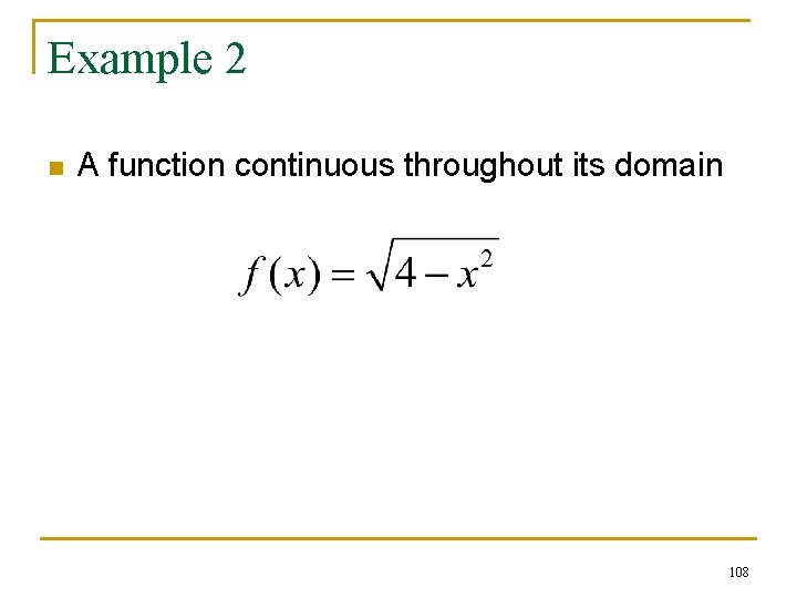
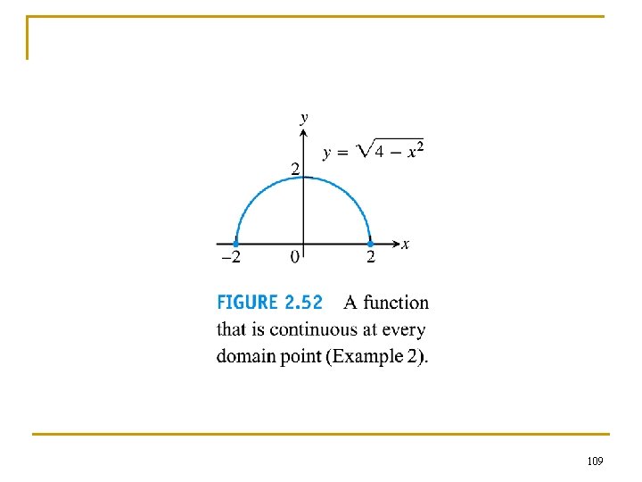
Example 2 n A function continuous throughout its domain 108
109
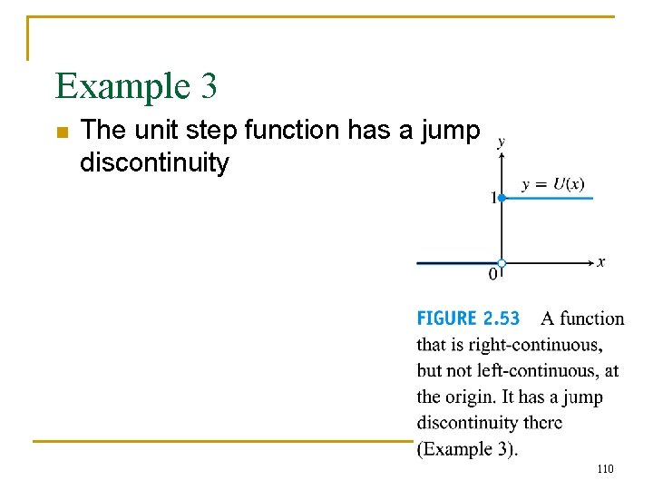
Example 3 n The unit step function has a jump discontinuity 110
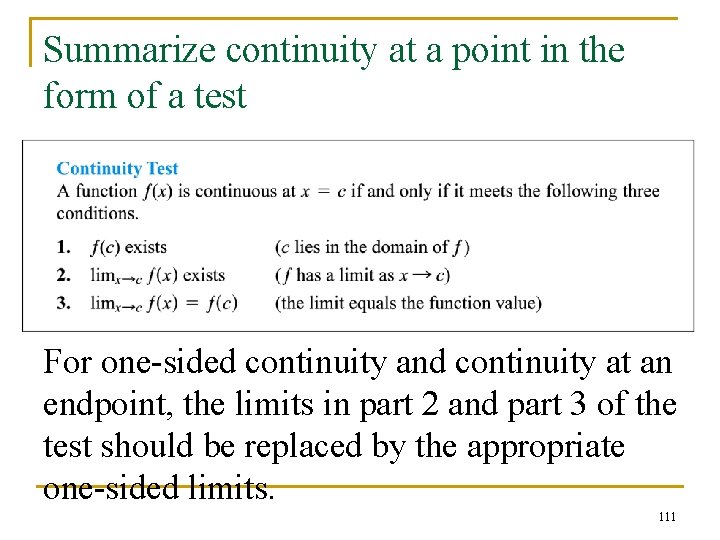
Summarize continuity at a point in the form of a test For one-sided continuity and continuity at an endpoint, the limits in part 2 and part 3 of the test should be replaced by the appropriate one-sided limits. 111
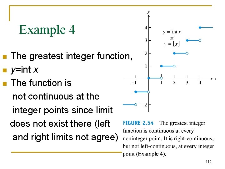
Example 4 n n n The greatest integer function, y=int x The function is not continuous at the integer points since limit does not exist there (left and right limits not agree) 112
113
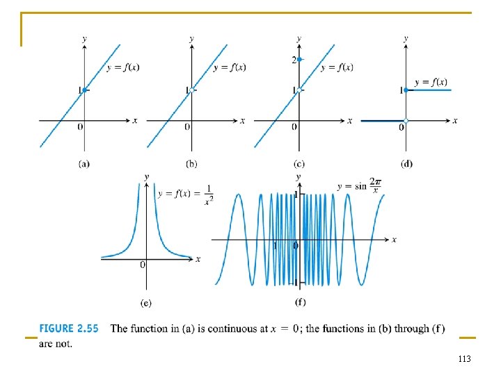
Discontinuity types n n (b), (c) removable discontinuity (d) jump discontinuity (e) infinite discontinuity (f) oscillating discontinuity 114
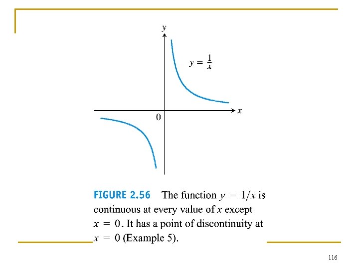
Continuous functions n n n A function is continuous on an interval if and only if it is continuous at every point of the interval. Example: Figure 2. 56 1/x not continuous on [-1, 1] but continuous over (-∞, 0) (0, ∞) 115
116
Example 5 n n Identifying continuous function (a) f(x)=1/x (b) f(x)= x Ask: is 1/x continuous over its domain? 117
118
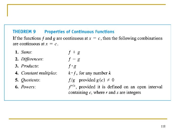
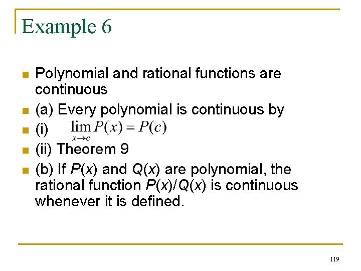
Example 6 n n n Polynomial and rational functions are continuous (a) Every polynomial is continuous by (i) (ii) Theorem 9 (b) If P(x) and Q(x) are polynomial, the rational function P(x)/Q(x) is continuous whenever it is defined. 119
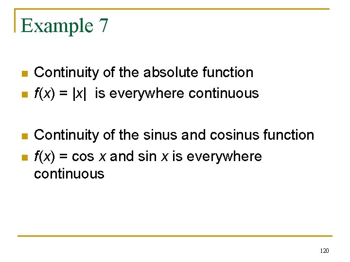
Example 7 n n Continuity of the absolute function f(x) = |x| is everywhere continuous Continuity of the sinus and cosinus function f(x) = cos x and sin x is everywhere continuous 120
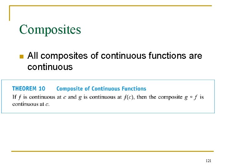
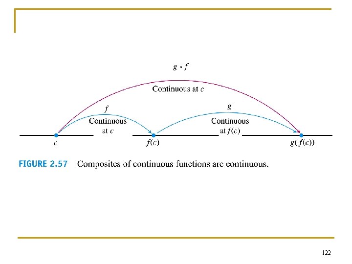
Composites n All composites of continuous functions are continuous 121
122
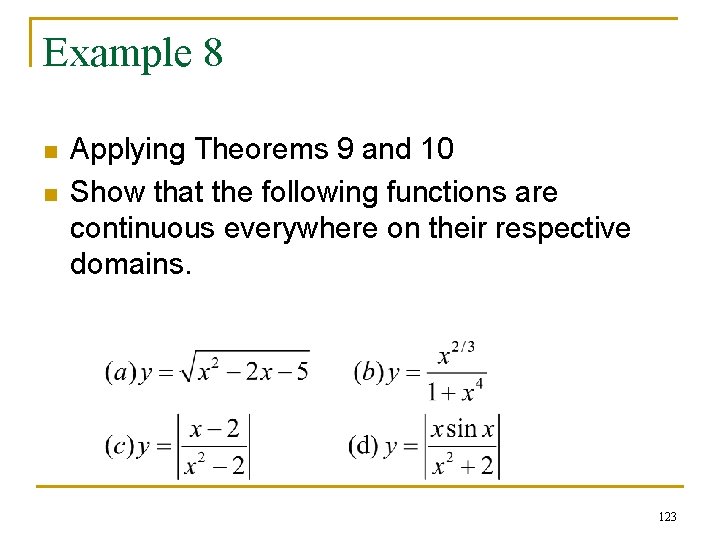
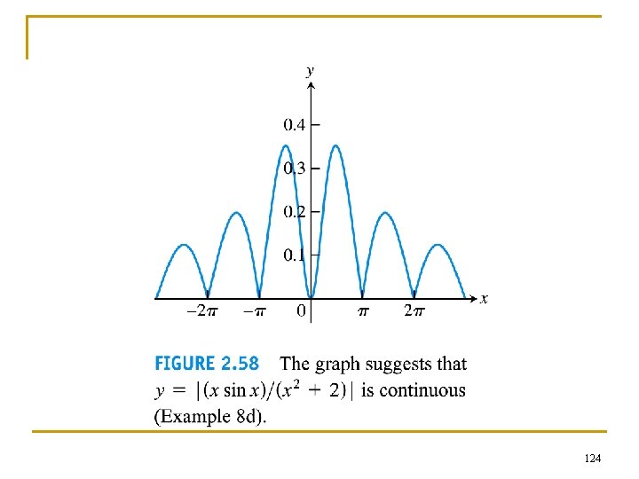
Example 8 n n Applying Theorems 9 and 10 Show that the following functions are continuous everywhere on their respective domains. 123
124
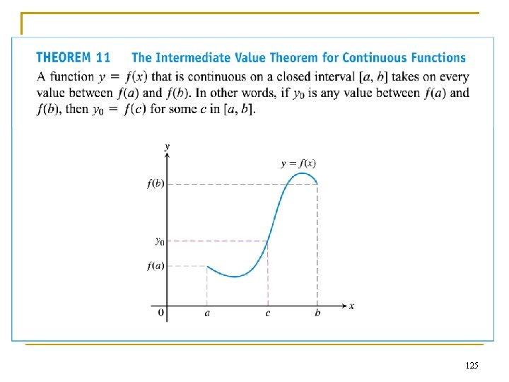
125
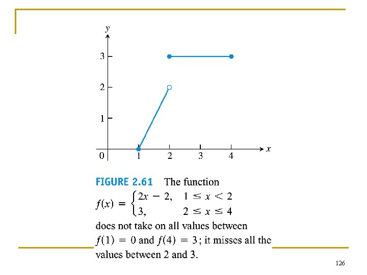
126
Consequence of root finding n n n A solution of the equation f(x)=0 is called a root. For example, f(x)= x 2 + x - 6, the roots are x=2, x=-3 since f(-3)=f(2)=0. Say f is continuous over some interval. Say a, b (with a < b) are in the domain of f, such that f(a) and f(b) have opposite signs. This means either f(a) < 0 < f(b) or f(b) < 0 < f(a) Then, as a consequence of theorem 11, there must exist at least a point c between a and b, i. e. a < c < b such that f(c)= 0. x=c is the root. 127
f(b)>0 y f(c)=0 f(a)<0 a c b x 128
Example n n n n Consider the function f(x) = x - cos x Prove that there is at least one root for f(x) in the interval [0, p/2]. Solution f(x) is continuous on (-∞, ∞). Say a = 0, b = p/2. f(x=0) = -1; f(x = p/2) = p/2 f(a) and f(b) have opposite signs Then, as a consequence of theorem 11, there must exist at least a point c between a and b, i. e. a=0 < c < b= p/2 such that f(c)= 0. x=c is the root. 129
2. 7 Tangents and Derivatives 130
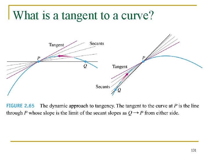
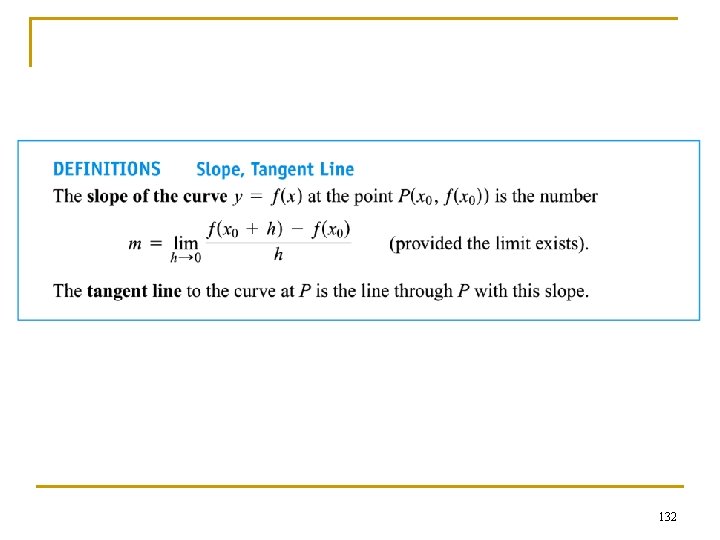
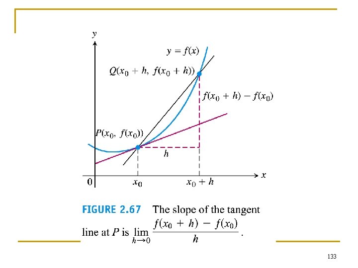
What is a tangent to a curve? 131
132
133
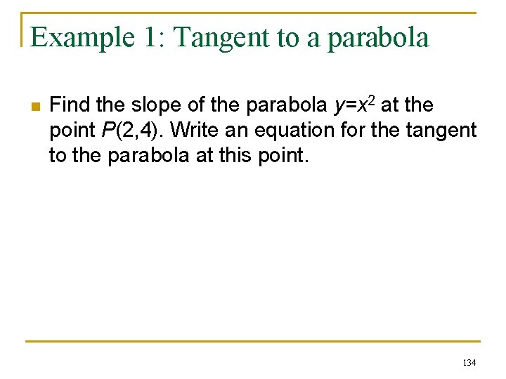
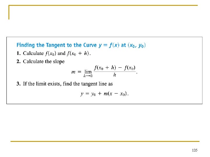
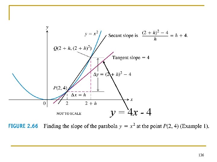
Example 1: Tangent to a parabola n Find the slope of the parabola y=x 2 at the point P(2, 4). Write an equation for the tangent to the parabola at this point. 134
135
y = 4 x - 4 136
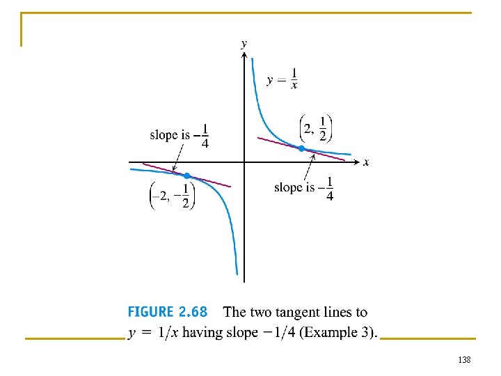
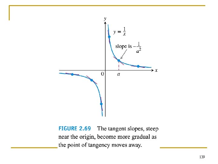
Example 3 n n Slope and tangent to y=1/x, x 0 (a) Find the slope of y=1/x at x = a 0 (b) Where does the slope equal -1/4? (c) What happens to the tangent of the curve at the point (a, 1/a) as a changes? 137
138
139