Analysis of Semisupervised Learning with the Yarowsky Algorithm

Analysis of Semi-supervised Learning with the Yarowsky Algorithm Gholamreza Haffari School of Computing Sciences Simon Fraser University

Outline Ø Introduction § Semi-supervised Learning, Self-training (Yarowsky Algorithm) Ø Bipartite Graph Representation § Yarowsky Algorithm on the Bipartite Graph Ø Analysing variants of the Yarowsky Algorithm § Objective Functions, Optimization Algorithms Ø Concluding Remarks 2

Outline Ø Introduction § Semi-supervised Learning, Self-training (Yarowsky Algorithm) Ø Bipartite Graph Representation § Yarowsky Algorithm on the Bipartite Graph Ø Analysing variants of the Yarowsky Algorithm § Objective Functions, Optimization Algorithms § Haffari & Sarkar, UAI, 2007. Ø Concluding Remarks 3

Outline Ø Introduction § Semi-supervised Learning, Self-training (Yarowsky Algorithm) Ø Bipartite Graph Representation § Yarowsky Algorithm on the Bipartite Graph Ø Analysing variants of the Yarowsky Algorithm § Objective Functions, Optimization Algorithms Ø Concluding Remarks 4

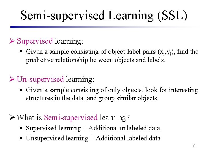
Semi-supervised Learning (SSL) Ø Supervised learning: § Given a sample consisting of object-label pairs (xi, yi), find the predictive relationship between objects and labels. Ø Un-supervised learning: § Given a sample consisting of only objects, look for interesting structures in the data, and group similar objects. Ø What is Semi-supervised learning? § Supervised learning + Additional unlabeled data § Unsupervised learning + Additional labeled data 5

Motivation for Semi-Supervised Learning (Belkin & Niyogi 2005) Ø Philosophical: § Human brain can exploit unlabeled data. Ø Pragmatic: § Unlabeled data is usually cheap to collect. 6

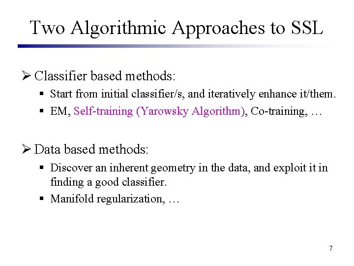
Two Algorithmic Approaches to SSL Ø Classifier based methods: § Start from initial classifier/s, and iteratively enhance it/them. § EM, Self-training (Yarowsky Algorithm), Co-training, … Ø Data based methods: § Discover an inherent geometry in the data, and exploit it in finding a good classifier. § Manifold regularization, … 7

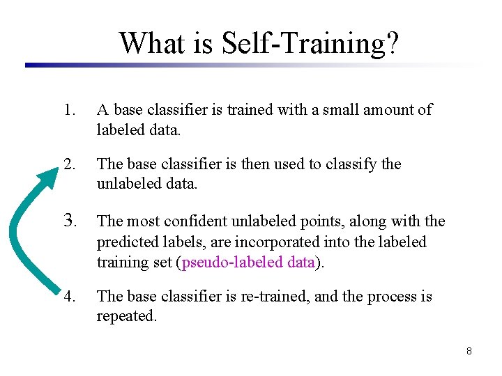
What is Self-Training? 1. A base classifier is trained with a small amount of labeled data. 2. The base classifier is then used to classify the unlabeled data. 3. The most confident unlabeled points, along with the predicted labels, are incorporated into the labeled training set (pseudo-labeled data). 4. The base classifier is re-trained, and the process is repeated. 8

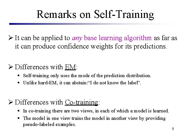
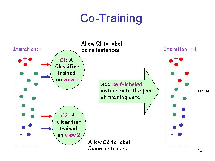
Remarks on Self-Training Ø It can be applied to any base learning algorithm as far as it can produce confidence weights for its predictions. Ø Differences with EM: § Self-training only uses the mode of the prediction distribution. § Unlike hard-EM, it can abstain: “I do not know the label”. Ø Differences with Co-training: § In co-training there are two views, in each of which a model is learned. § The model in one view trains the model in another view by providing pseudo-labeled examples. 9

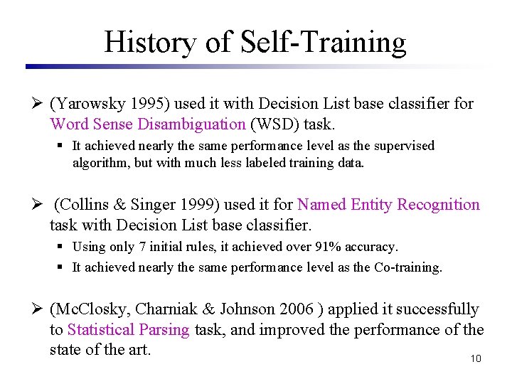
History of Self-Training Ø (Yarowsky 1995) used it with Decision List base classifier for Word Sense Disambiguation (WSD) task. § It achieved nearly the same performance level as the supervised algorithm, but with much less labeled training data. Ø (Collins & Singer 1999) used it for Named Entity Recognition task with Decision List base classifier. § Using only 7 initial rules, it achieved over 91% accuracy. § It achieved nearly the same performance level as the Co-training. Ø (Mc. Closky, Charniak & Johnson 2006 ) applied it successfully to Statistical Parsing task, and improved the performance of the state of the art. 10

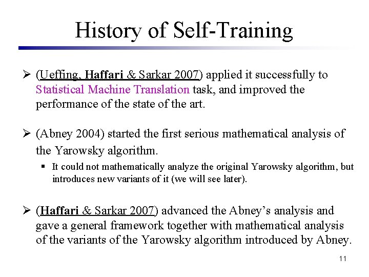
History of Self-Training Ø (Ueffing, Haffari & Sarkar 2007) applied it successfully to Statistical Machine Translation task, and improved the performance of the state of the art. Ø (Abney 2004) started the first serious mathematical analysis of the Yarowsky algorithm. § It could not mathematically analyze the original Yarowsky algorithm, but introduces new variants of it (we will see later). Ø (Haffari & Sarkar 2007) advanced the Abney’s analysis and gave a general framework together with mathematical analysis of the variants of the Yarowsky algorithm introduced by Abney. 11

Outline Ø Introduction § Semi-supervised Learning, Self-training (Yarowsky Algorithm) Ø Bipartite Graph Representation § Yarowsky Algorithm on the Bipartite Graph Ø Analysing variants of the Yarowsky Algorithm § Objective Functions, Optimization Algorithms Ø Concluding Remarks 12

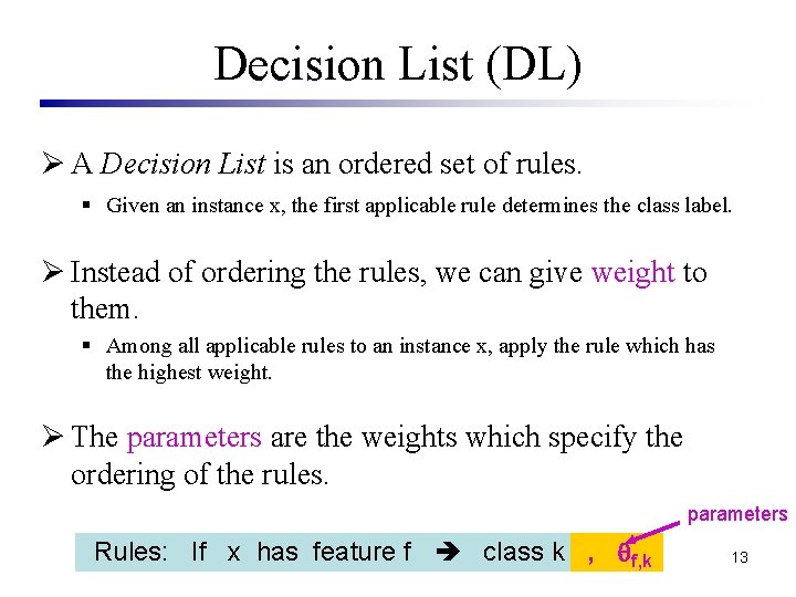
Decision List (DL) Ø A Decision List is an ordered set of rules. § Given an instance x, the first applicable rule determines the class label. Ø Instead of ordering the rules, we can give weight to them. § Among all applicable rules to an instance x, apply the rule which has the highest weight. Ø The parameters are the weights which specify the ordering of the rules. parameters Rules: If x has feature f class k , f, k 13

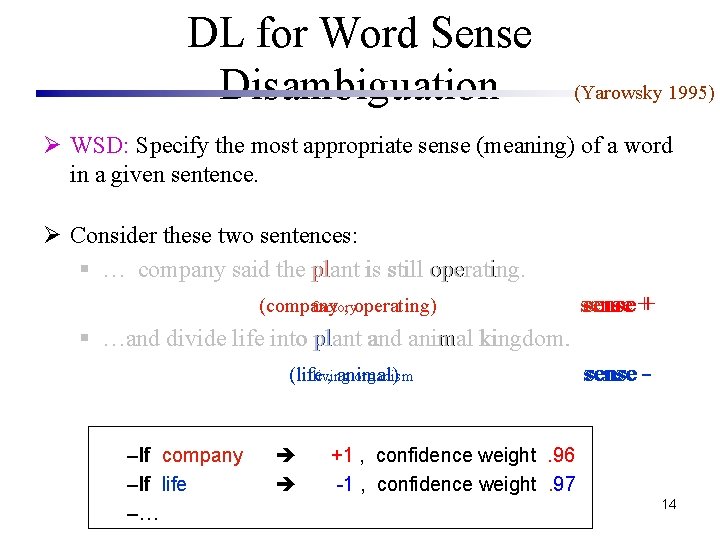
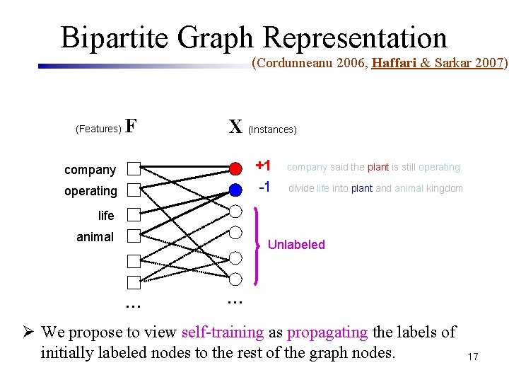
DL for Word Sense Disambiguation (Yarowsky 1995) Ø WSD: Specify the most appropriate sense (meaning) of a word in a given sentence. Ø Consider these two sentences: § … company said the plant is still operating. (company factory , operating) sense ++ § …and divide life into plant and animal kingdom. (lifeliving , animal) organism –If company –If life –… sense -- +1 , confidence weight. 96 -1 , confidence weight. 97 14

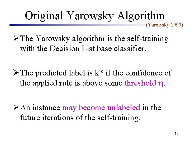
Original Yarowsky Algorithm (Yarowsky 1995) Ø The Yarowsky algorithm is the self-training with the Decision List base classifier. Ø The predicted label is k* if the confidence of the applied rule is above some threshold . Ø An instance may become unlabeled in the future iterations of the self-training. 15

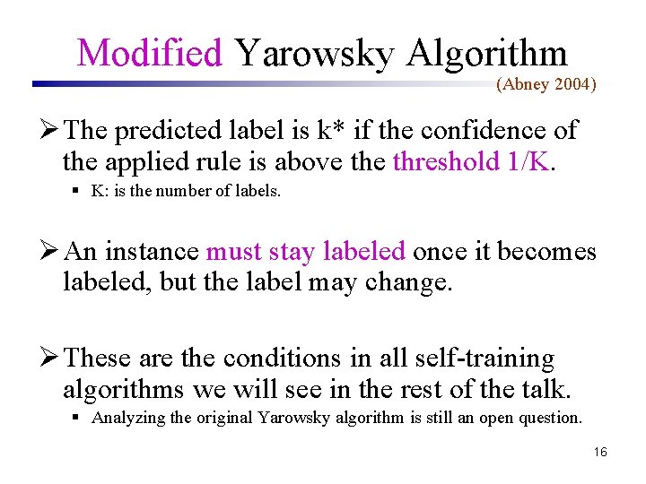
Modified Yarowsky Algorithm (Abney 2004) Ø The predicted label is k* if the confidence of the applied rule is above threshold 1/K. § K: is the number of labels. Ø An instance must stay labeled once it becomes labeled, but the label may change. Ø These are the conditions in all self-training algorithms we will see in the rest of the talk. § Analyzing the original Yarowsky algorithm is still an open question. 16

Bipartite Graph Representation (Cordunneanu 2006, Haffari & Sarkar 2007) (Features) F X (Instances) +1 -1 company operating company said the plant is still operating divide life into plant and animal kingdom life animal Unlabeled … … Ø We propose to view self-training as propagating the labels of initially labeled nodes to the rest of the graph nodes. 17

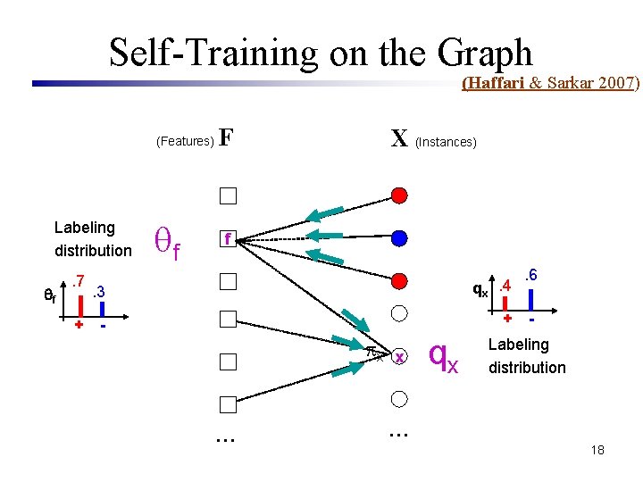
Self-Training on the Graph (Haffari & Sarkar 2007) (Features) Labeling distribution f . 7 + f F X (Instances) f . 3 qx. 4 - + x … x qx . 6 - Labeling distribution … 18

Outline (Haffari & Sarkar 2007) Ø Introduction § Semi-supervised Learning, Self-training (Yarowsky Algorithm) Ø Bipartite Graph Representation § Yarowsky Algorithm on the Bipartite Graph Ø Analysing variants of the Yarowsky Algorithm § Objective Functions, Optimization Algorithms Ø Concluding Remarks 19

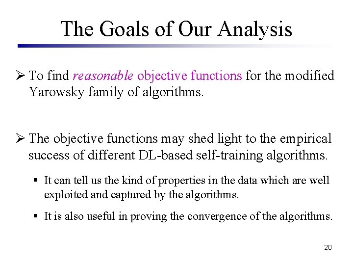
The Goals of Our Analysis Ø To find reasonable objective functions for the modified Yarowsky family of algorithms. Ø The objective functions may shed light to the empirical success of different DL-based self-training algorithms. § It can tell us the kind of properties in the data which are well exploited and captured by the algorithms. § It is also useful in proving the convergence of the algorithms. 20

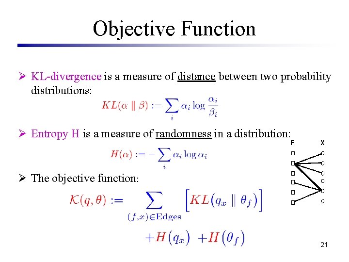
Objective Function Ø KL-divergence is a measure of distance between two probability distributions: Ø Entropy H is a measure of randomness in a distribution: F X Ø The objective function: 21

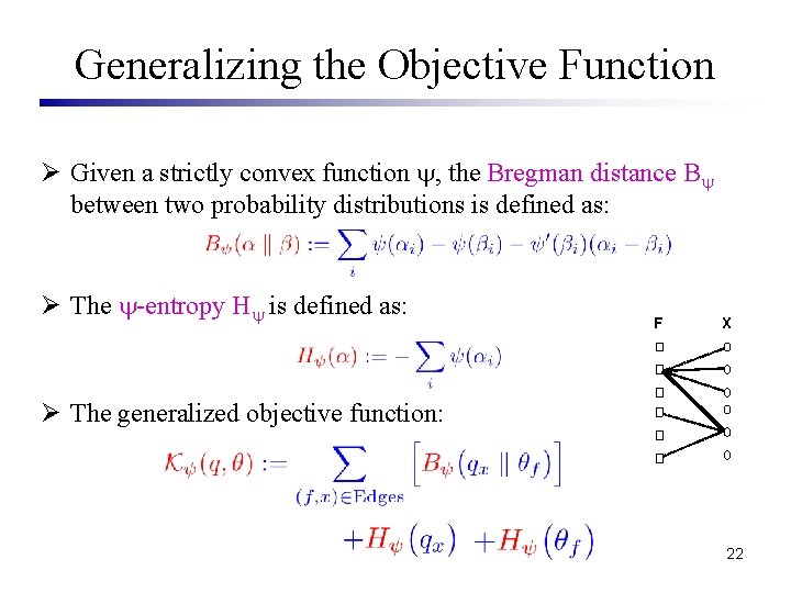
Generalizing the Objective Function Ø Given a strictly convex function , the Bregman distance B between two probability distributions is defined as: Ø The -entropy H is defined as: F X Ø The generalized objective function: 22

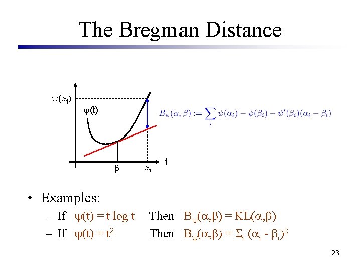
The Bregman Distance ( i) (t) i i t • Examples: – If (t) = t log t – If (t) = t 2 Then B ( , ) = KL( , ) Then B ( , ) = i ( i - i)2 23

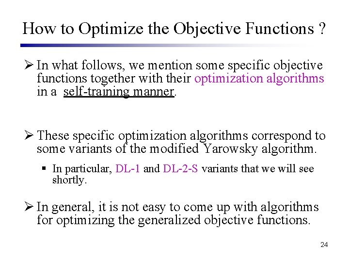
How to Optimize the Objective Functions ? Ø In what follows, we mention some specific objective functions together with their optimization algorithms in a self-training manner. Ø These specific optimization algorithms correspond to some variants of the modified Yarowsky algorithm. § In particular, DL-1 and DL-2 -S variants that we will see shortly. Ø In general, it is not easy to come up with algorithms for optimizing the generalized objective functions. 24

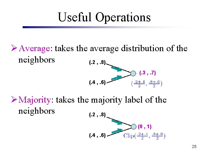
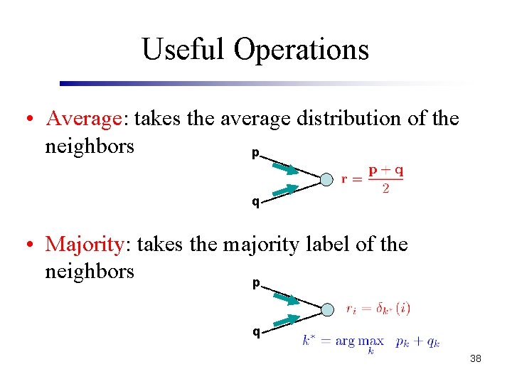
Useful Operations Ø Average: takes the average distribution of the neighbors (. 2 , . 8) (. 3 , . 7) (. 4 , . 6) Ø Majority: takes the majority label of the neighbors (. 2 , . 8) (0 , 1) (. 4 , . 6) 25

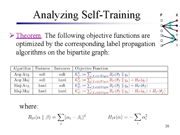
Analyzing Self-Training F X Ø Theorem. The following objective functions are optimized by the corresponding label propagation algorithms on the bipartite graph: where: 26

Remarks on the Theorem Ø The final solution of the Average-Average algorithm is related to the graph-based semi-supervised learning using harmonic functions (Zhu et al 2003). Ø The Average-Majority algorithm is the so-called DL-1 variant of the modified Yarowsky algorithm. Ø We can show that the Majority-Majority algorithm converges in polynomial-time O(|F|2. |X|2). 27

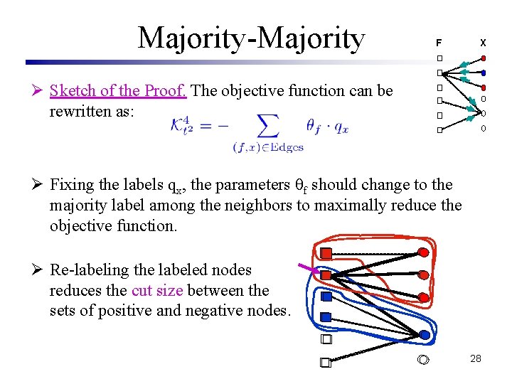
Majority-Majority F X Ø Sketch of the Proof. The objective function can be rewritten as: Ø Fixing the labels qx, the parameters f should change to the majority label among the neighbors to maximally reduce the objective function. Ø Re-labeling the labeled nodes reduces the cut size between the sets of positive and negative nodes. 28

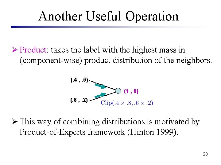
Another Useful Operation Ø Product: takes the label with the highest mass in (component-wise) product distribution of the neighbors. (. 4 , . 6) (1 , 0) (. 8 , . 2) Ø This way of combining distributions is motivated by Product-of-Experts framework (Hinton 1999). 29

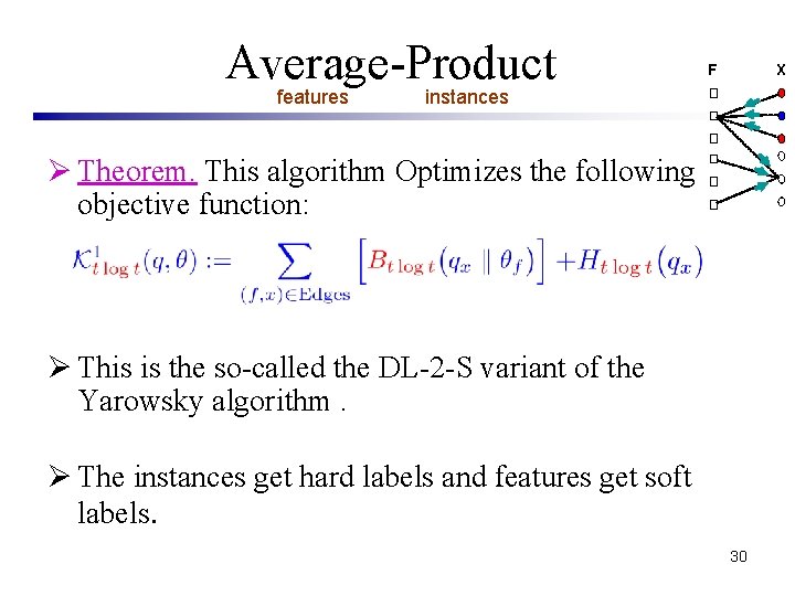
Average-Product features F X instances Ø Theorem. This algorithm Optimizes the following objective function: Ø This is the so-called the DL-2 -S variant of the Yarowsky algorithm. Ø The instances get hard labels and features get soft labels. 30

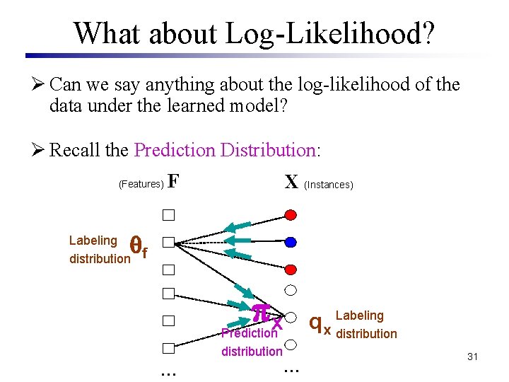
What about Log-Likelihood? Ø Can we say anything about the log-likelihood of the data under the learned model? Ø Recall the Prediction Distribution: (Features) F X (Instances) Labeling distribution f x Prediction distribution … qx Labeling distribution … 31

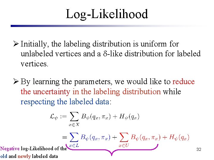
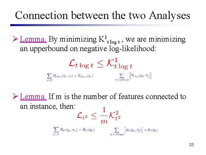
Log-Likelihood Ø Initially, the labeling distribution is uniform for unlabeled vertices and a -like distribution for labeled vertices. Ø By learning the parameters, we would like to reduce the uncertainty in the labeling distribution while respecting the labeled data: Negative log-Likelihood of the old and newly labeled data 32

Connection between the two Analyses Ø Lemma. By minimizing K 1 t log t , we are minimizing an upperbound on negative log-likelihood: Ø Lemma. If m is the number of features connected to an instance, then: 33

Outline Ø Introduction § Semi-supervised Learning, Self-training, Yarowsky Algorithm Ø Problem Formulation § Bipartite-graph Representation, Modified Yarowsky family of Algorithms Ø Analysing variants of the Yarowsky Algorithm § Objective Functions, Optimization Algorithms Ø Concluding Remarks 34

Summary Ø We have reviewed variants of the Yarowsky algorithms for rulebased semi-supervised learning. Ø We have proposed a general framework to unify and analyze variants of the Yarowsky algorithm and some other semisupervised learning algorithms. It allows us to: § introduce new self-training style algorithms. § shed light to the reasons of the success of some of the existing bootstrapping algorithms. Ø Still there exist important and interesting un-answered questions which are avenues for future research. 35

Thank You 36

References Ø Belkin & Niyogi, Chicago Machine Learning Summer School, 2005. Ø D. Yarowsky, Unsupervised Word Sense Disambiguation Rivaling Supervised Methods, ACL, 1995. Ø M. Collins and Y. Singer, Unsupervised Models for Named Entity Classification, EMNLP, 1999. Ø D. Mc. Closky, E. Charniak, and M. Johnson, Reranking and Self-Training for Parser Adaptation, COLING-ACL, 2006. Ø G. Haffari, A. Sarkar, Analysis of Semi-Supervised Learning with the Yarowsky Algorithm, UAI, 2007. Ø N. Ueffing, G. Haffari, A. Sarkar, Transductive Learning for Statistical Machine Translation, ACL, 2007. Ø S. Abney, Understanding the Yarowsky Algorithm, Computational Linguistics 30(3). 2004. Ø A. Corduneanu, The Information Regularization Framework for Semi-Supervised Learning, Ph. D. thesis, MIT, 2006. Ø M. Balan, and A. Blum, An Augmented PAC Model for Semi-Supervised Learning, Book Chapter in Semi-Supervised Learning, MIT Press, 2006. Ø J. Eisner and D. Karakos, Bootstrapping Without the Boot, HLT-EMNLP, 2005. 37

Useful Operations • Average: takes the average distribution of the neighbors p q • Majority: takes the majority label of the neighbors p q 38

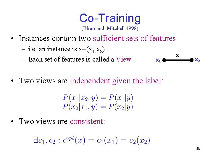
Co-Training (Blum and Mitchell 1998) • Instances contain two sufficient sets of features – i. e. an instance is x=(x 1, x 2) – Each set of features is called a View x 1 x x 2 • Two views are independent given the label: • Two views are consistent: 39

Co-Training Allow C 1 to label Some instances Iteration: t + - C 1: A Classifier trained on view 1 C 2: A Classifier trained on view 2 Iteration: t+1 + Add self-labeled instances to the pool of training data …… Allow C 2 to label Some instances 40