ANALYSIS AND DESIGN OF ALGORITHMS UNITII CHAPTER 4

ANALYSIS AND DESIGN OF ALGORITHMS UNIT-II CHAPTER 4: DIVIDE –AND- CONQUER 1

OUTLINE Ø Divide – and - Conquer Technique • • Merge sort Quick sort Binary Search Multiplication of Large Integers and Strassen’s Matrix Multiplication 2

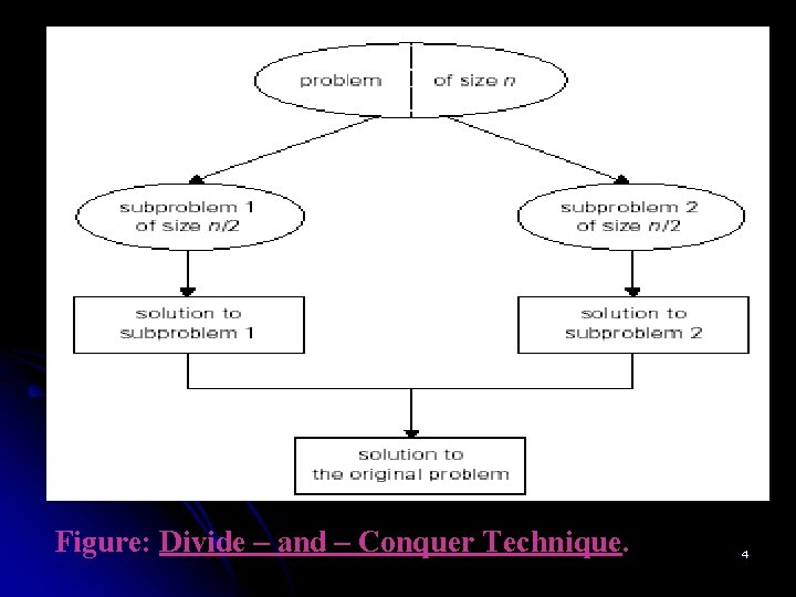
Divide – and – Conquer : Divide – and - conquer algorithms work according to the following general plan : 1. A problem’s instance is divided into several smaller instances of the same problem, ideally of about the same size. 2. The smaller instances are solved (typically recursively). 3. The solutions obtained for the smaller instances are combined to get a solution to the original problem. 3

Figure: Divide – and – Conquer Technique. 4

Divide – and – Conquer : Ø Not every divide-and-conquer algorithm is necessarily more efficient than even a brute-force solution. Ø The divide-and-conquer approach yields some of the most important and efficient algorithms in computer science. Ø Divide-and-Conquer technique is ideally suited for parallel computations, in which each subproblem can be solved simultaneously by its own processor. Later all solutions can be merged to get solution to original problem. Thus, the execution speed of a program which is based on this technique can be improved significantly. 5

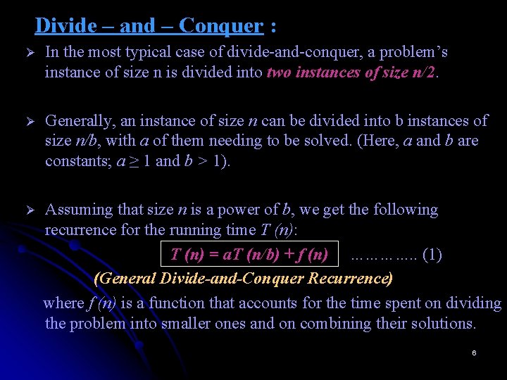
Divide – and – Conquer : Ø In the most typical case of divide-and-conquer, a problem’s instance of size n is divided into two instances of size n/2. Ø Generally, an instance of size n can be divided into b instances of size n/b, with a of them needing to be solved. (Here, a and b are constants; a ≥ 1 and b > 1). Ø Assuming that size n is a power of b, we get the following recurrence for the running time T (n): T (n) = a. T (n/b) + f (n) …………. . (1) (General Divide-and-Conquer Recurrence) where f (n) is a function that accounts for the time spent on dividing the problem into smaller ones and on combining their solutions. 6

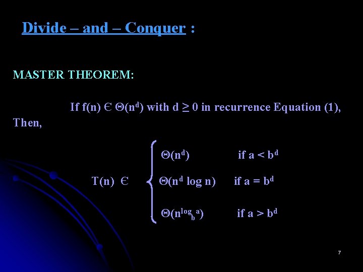
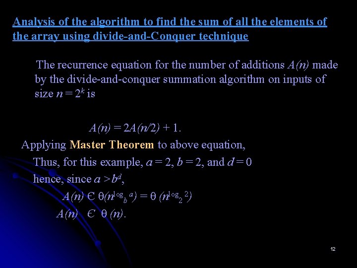
Divide – and – Conquer : MASTER THEOREM: If f(n) Є Θ(nd) with d ≥ 0 in recurrence Equation (1), Then, Θ(nd) T(n) Є if a < bd Θ(nd log n) if a = bd Θ(nlogba) if a > bd 7

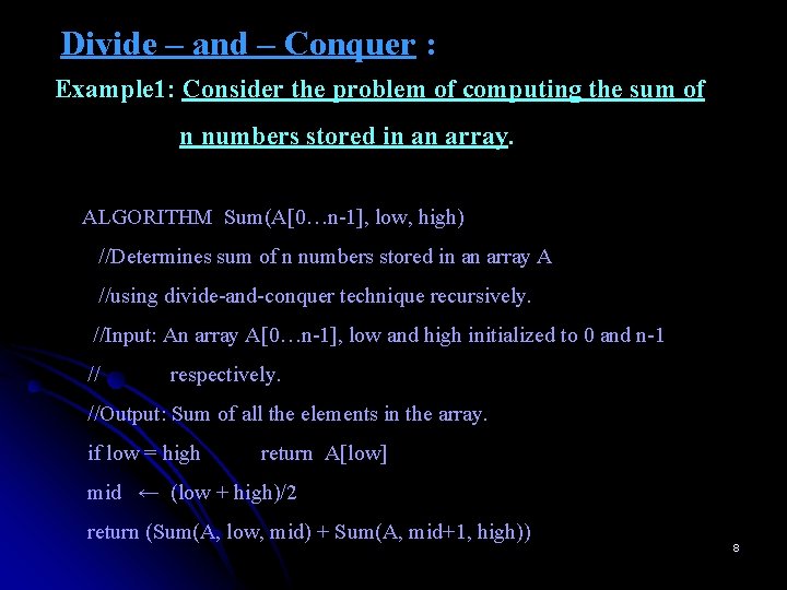
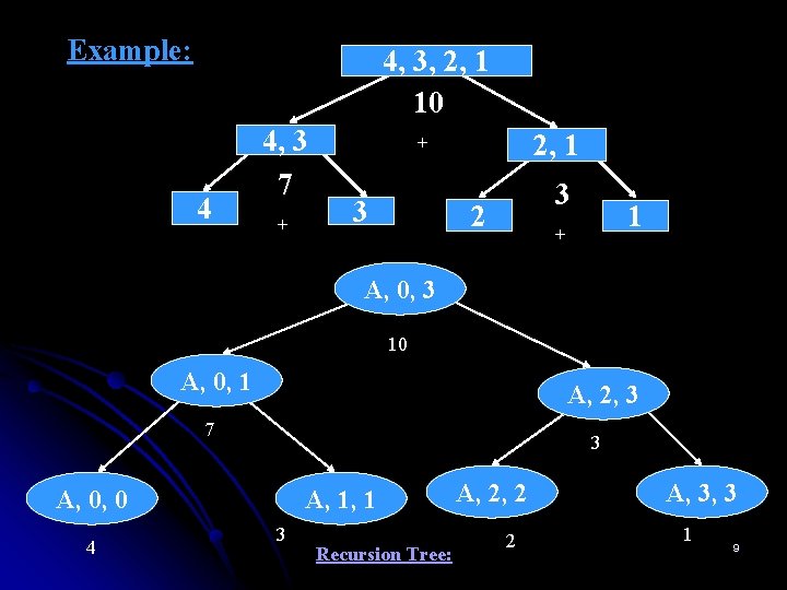
Divide – and – Conquer : Example 1: Consider the problem of computing the sum of n numbers stored in an array. ALGORITHM Sum(A[0…n-1], low, high) //Determines sum of n numbers stored in an array A //using divide-and-conquer technique recursively. //Input: An array A[0…n-1], low and high initialized to 0 and n-1 // respectively. //Output: Sum of all the elements in the array. if low = high return A[low] mid ← (low + high)/2 return (Sum(A, low, mid) + Sum(A, mid+1, high)) 8

Example: 4, 3, 2, 1 10 4 4, 3 7 + 2, 1 + 3 3 2 1 + A, 0, 3 10 A, 0, 1 A, 2, 3 7 3 A, 0, 0 4 A, 1, 1 3 Recursion Tree: A, 2, 2 2 A, 3, 3 1 9

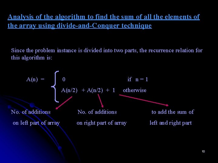
Analysis of the algorithm to find the sum of all the elements of the array using divide-and-Conquer technique Since the problem instance is divided into two parts, the recurrence relation for this algorithm is: A(n) = 0 if n = 1 A(n/2) + 1 otherwise No. of additions on left part of array on right part of array to add the sum of left and right part 10

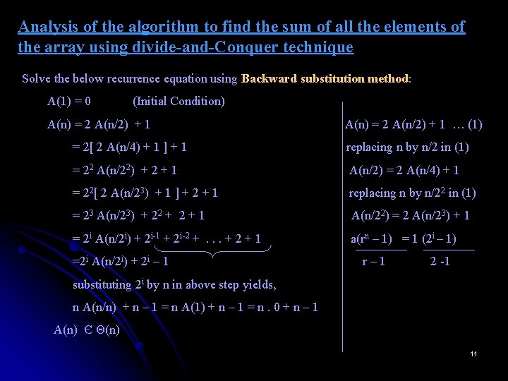
Analysis of the algorithm to find the sum of all the elements of the array using divide-and-Conquer technique Solve the below recurrence equation using Backward substitution method: A(1) = 0 (Initial Condition) A(n) = 2 A(n/2) + 1 … (1) = 2[ 2 A(n/4) + 1 ] + 1 replacing n by n/2 in (1) = 22 A(n/22) + 2 + 1 A(n/2) = 2 A(n/4) + 1 = 22[ 2 A(n/23) + 1 ] + 2 + 1 replacing n by n/22 in (1) = 23 A(n/23) + 22 + 1 A(n/22) = 2 A(n/23) + 1 = 2 i A(n/2 i) + 2 i-1 + 2 i-2 +. . . + 2 + 1 a(rn – 1) = 1 (2 i – 1) =2 i A(n/2 i) + 2 i – 1 r– 1 2 -1 substituting 2 i by n in above step yields, n A(n/n) + n – 1 = n A(1) + n – 1 = n. 0 + n – 1 A(n) Є Θ(n) 11

Analysis of the algorithm to find the sum of all the elements of the array using divide-and-Conquer technique The recurrence equation for the number of additions A(n) made by the divide-and-conquer summation algorithm on inputs of size n = 2 k is A(n) = 2 A(n/2) + 1. Applying Master Theorem to above equation, Thus, for this example, a = 2, b = 2, and d = 0 hence, since a >bd, A(n) Є θ(nlogb a) = θ (nlog 2 2) A(n) Є θ (n). 12

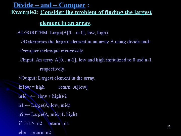
Divide – and – Conquer : Example 2: Consider the problem of finding the largest element in an array. ALGORITHM Large(A[0…n-1], low, high) //Determines the largest element in an array A using divide-and//conquer technique recursively. //Input: An array A[0…n-1], low and high initialized to 0 and n-1 respectively. //Output: Largest element in the array. if low = high return A[low] mid ← (low + high)/2 n 1 ← Large(A, low, mid) n 2 ← Large(A, mid+1, high) if n 1 > n 2 return n 1 else return n 2 13

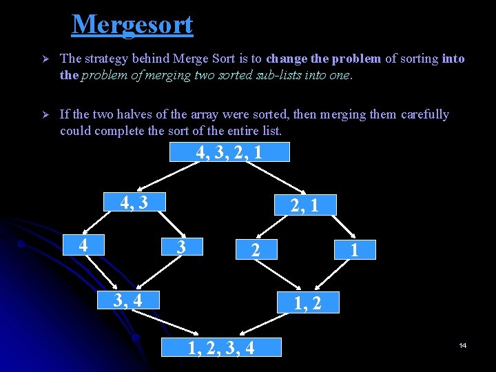
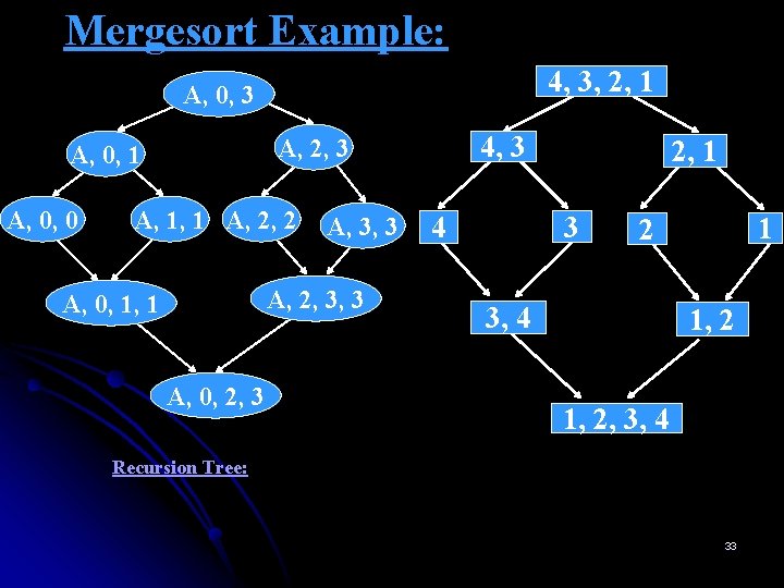
Mergesort Ø The strategy behind Merge Sort is to change the problem of sorting into the problem of merging two sorted sub-lists into one. Ø If the two halves of the array were sorted, then merging them carefully could complete the sort of the entire list. 4, 3, 2, 1 4, 3 4 2, 1 3 2 3, 4 1 1, 2, 3, 4 14

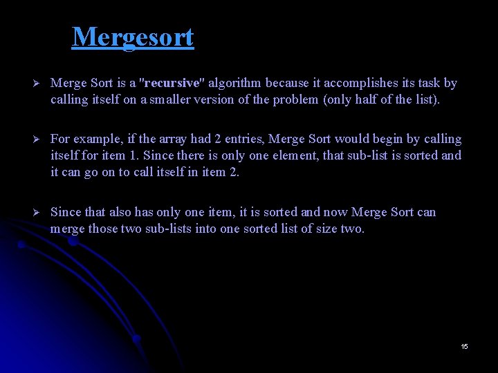
Mergesort Ø Merge Sort is a "recursive" algorithm because it accomplishes its task by calling itself on a smaller version of the problem (only half of the list). Ø For example, if the array had 2 entries, Merge Sort would begin by calling itself for item 1. Since there is only one element, that sub-list is sorted and it can go on to call itself in item 2. Ø Since that also has only one item, it is sorted and now Merge Sort can merge those two sub-lists into one sorted list of size two. 15

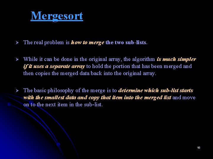
Mergesort Ø The real problem is how to merge the two sub-lists. Ø While it can be done in the original array, the algorithm is much simpler if it uses a separate array to hold the portion that has been merged and then copies the merged data back into the original array. Ø The basic philosophy of the merge is to determine which sub-list starts with the smallest data and copy that item into the merged list and move on to the next item in the sub-list. 16

Mergesort ALGORITHM Mergesort(A[0…n-1]) //Sorts array A[0…n-1] by recursive mergesort //Input: An array A[0…n-1] of orderable elements //Output: Array A[0…n-1] sorted in nondecreasing order if n > 1 copy A[0. . . n/2 - 1] to B[0. . . n/2 - 1] copy A[ n/2. . . n - 1] to C[0. . . n/2 – 1] Mergesort(B[0. . . n/2 – 1]) Mergesort(C[0. . . n/2 – 1]) Merge(B, C, A) 17

Mergesort ALGORITHM Merge(B[0. . . p-1], C[0. . . q-1], A[0. . . p + q - 1]) //Merges two sorted arrays into one sorted array //Input: Arrays B[0. . . p-1] and C[0. . . q-1] both sorted //Output: Sorted array A[0. . . p + q - 1] of the elements of B & C i ← 0, j ← 0, k ← 0 while i < p and j < q do if B[i] ≤ C[j] A[k] ← B[i]; i ← i + 1 else A[k] ← C[j]; j ← j + 1 k←k+1 if i = p copy C[j. . . q – 1] to A[k. . . p + q – 1] else copy B[i. . . p – 1] to A[k. . . p + q – 1] 18

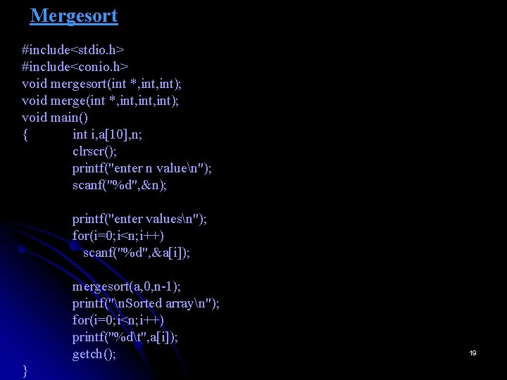
Mergesort #include<stdio. h> #include<conio. h> void mergesort(int *, int); void merge(int *, int, int); void main() { int i, a[10], n; clrscr(); printf("enter n valuen"); scanf("%d", &n); printf("enter valuesn"); for(i=0; i<n; i++) scanf("%d", &a[i]); mergesort(a, 0, n-1); printf("n. Sorted arrayn"); for(i=0; i<n; i++) printf("%dt", a[i]); getch(); } 19

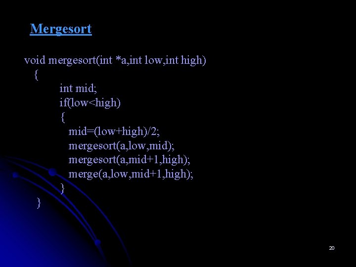
Mergesort void mergesort(int *a, int low, int high) { int mid; if(low<high) { mid=(low+high)/2; mergesort(a, low, mid); mergesort(a, mid+1, high); merge(a, low, mid+1, high); } } 20

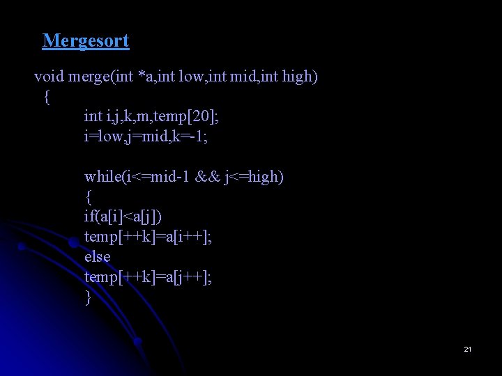
Mergesort void merge(int *a, int low, int mid, int high) { int i, j, k, m, temp[20]; i=low, j=mid, k=-1; while(i<=mid-1 && j<=high) { if(a[i]<a[j]) temp[++k]=a[i++]; else temp[++k]=a[j++]; } 21

Mergesort // copy remaining elements into temp array for(m=i; m<=mid-1; m++) temp[++k]=a[m]; for(m=j; m<=high; m++) temp[++k]=a[m]; // copy elements of temp array back into array a for(m=0; m<=k; m++) a[low+m]=temp[m]; } 22

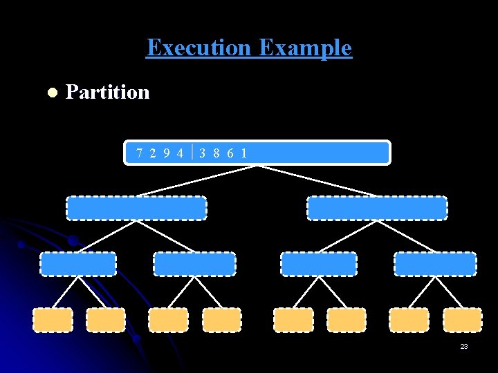
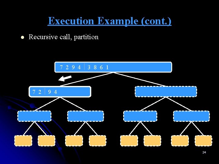
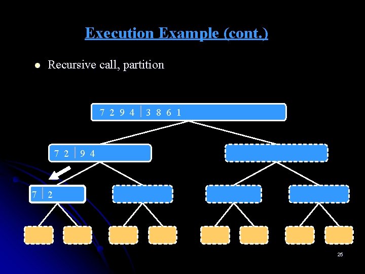
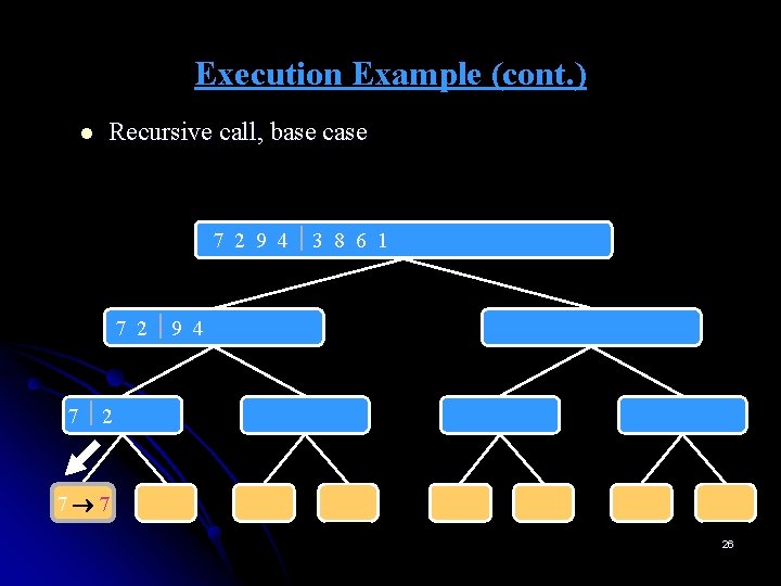
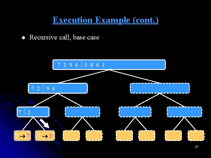
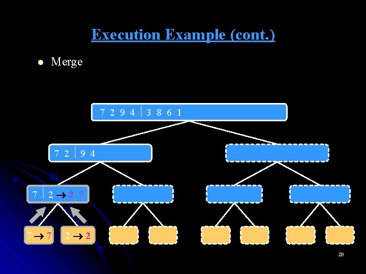
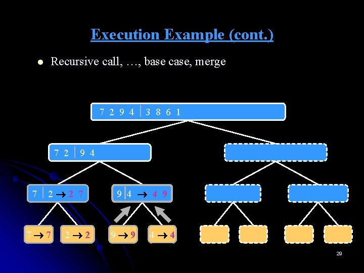
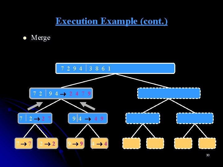
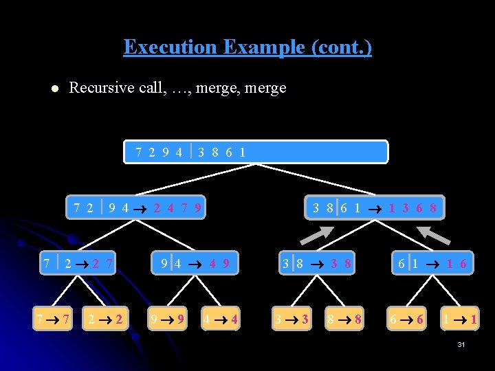
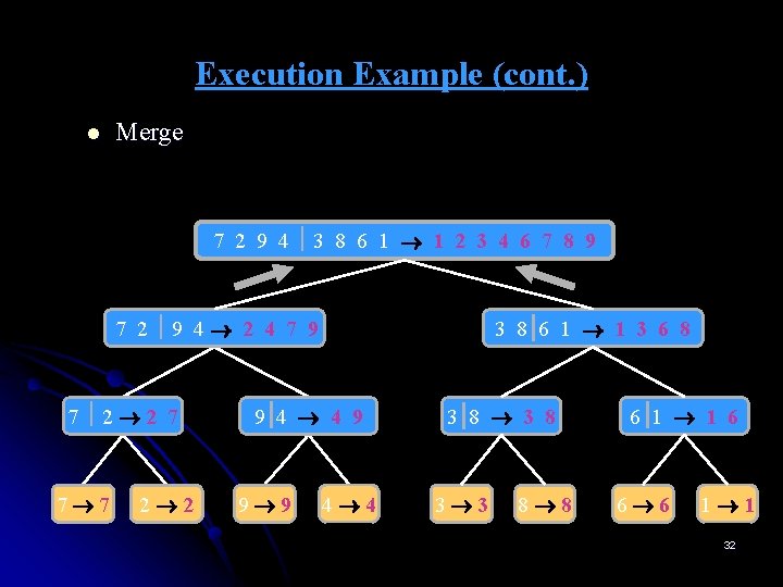
Execution Example l Partition 7 2 9 4 3 8 6 1 1 2 3 4 6 7 8 9 7 2 9 4 2 4 7 9 7 2 2 7 7 7 2 2 3 8 6 1 1 3 8 6 9 4 4 9 9 9 4 4 3 8 3 3 8 8 6 1 1 6 6 6 1 1 23

Execution Example (cont. ) l Recursive call, partition 7 2 9 4 3 8 6 1 1 2 3 4 6 7 8 9 7 2 9 4 2 4 7 9 7 2 2 7 7 7 2 2 3 8 6 1 1 3 8 6 9 4 4 9 9 9 4 4 3 8 3 3 8 8 6 1 1 6 6 6 1 1 24

Execution Example (cont. ) l Recursive call, partition 7 2 9 4 3 8 6 1 1 2 3 4 6 7 8 9 7 2 9 4 2 4 7 9 7 2 2 7 7 7 2 2 3 8 6 1 1 3 8 6 9 4 4 9 9 9 4 4 3 8 3 3 8 8 6 1 1 6 6 6 1 1 25

Execution Example (cont. ) l Recursive call, base case 7 2 9 4 3 8 6 1 1 2 3 4 6 7 8 9 7 2 9 4 2 4 7 9 7 2 2 7 7 7 2 2 3 8 6 1 1 3 8 6 9 4 4 9 9 9 4 4 3 8 3 3 8 8 6 1 1 6 6 6 1 1 26

Execution Example (cont. ) l Recursive call, base case 7 2 9 4 3 8 6 1 1 2 3 4 6 7 8 9 7 2 9 4 2 4 7 9 7 2 2 7 7 7 2 2 3 8 6 1 1 3 8 6 9 4 4 9 9 9 4 4 3 8 3 3 8 8 6 1 1 6 6 6 1 1 27

Execution Example (cont. ) l Merge 7 2 9 4 3 8 6 1 1 2 3 4 6 7 8 9 7 2 9 4 2 4 7 9 7 2 2 7 7 7 2 2 3 8 6 1 1 3 8 6 9 4 4 9 9 9 4 4 3 8 3 3 8 8 6 1 1 6 6 6 1 1 28

Execution Example (cont. ) l Recursive call, …, base case, merge 7 2 9 4 3 8 6 1 1 2 3 4 6 7 8 9 7 2 9 4 2 4 7 9 7 2 2 7 7 7 2 2 3 8 6 1 1 3 8 6 9 4 4 9 9 9 4 4 3 8 3 3 8 8 6 1 1 6 6 6 1 1 29

Execution Example (cont. ) l Merge 7 2 9 4 3 8 6 1 1 2 3 4 6 7 8 9 7 2 9 4 2 4 7 9 7 2 2 7 7 7 2 2 3 8 6 1 1 3 8 6 9 4 4 9 9 9 4 4 3 8 3 3 8 8 6 1 1 6 6 6 1 1 30

Execution Example (cont. ) l Recursive call, …, merge 7 2 9 4 3 8 6 1 1 2 3 4 6 7 8 9 7 2 9 4 2 4 7 9 7 2 2 7 7 7 2 2 3 8 6 1 1 3 6 8 9 4 4 9 9 9 4 4 3 8 3 3 8 8 6 1 1 6 6 6 1 1 31

Execution Example (cont. ) l Merge 7 2 9 4 3 8 6 1 1 2 3 4 6 7 8 9 7 2 9 4 2 4 7 9 7 2 2 7 7 7 2 2 3 8 6 1 1 3 6 8 9 4 4 9 9 9 4 4 3 8 3 3 8 8 6 1 1 6 6 6 1 1 32

Mergesort Example: 4, 3, 2, 1 A, 0, 3 A, 0, 0 4, 3 A, 2, 3 A, 0, 1 A, 1, 1 A, 2, 2 A, 3, 3 A, 2, 3, 3 A, 0, 1, 1 A, 0, 2, 3 2, 1 3 4 1 2 3, 4 1, 2, 3, 4 Recursion Tree: 33

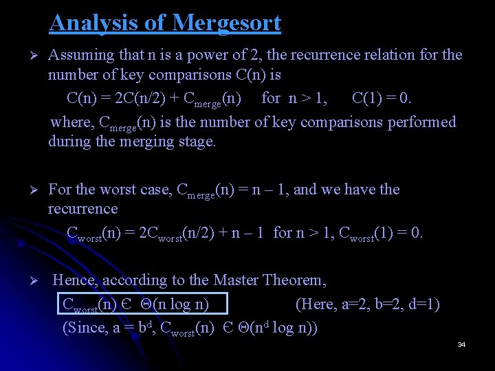
Analysis of Mergesort Ø Assuming that n is a power of 2, the recurrence relation for the number of key comparisons C(n) is C(n) = 2 C(n/2) + Cmerge(n) for n > 1, C(1) = 0. where, Cmerge(n) is the number of key comparisons performed during the merging stage. Ø For the worst case, Cmerge(n) = n – 1, and we have the recurrence Cworst(n) = 2 Cworst(n/2) + n – 1 for n > 1, Cworst(1) = 0. Ø Hence, according to the Master Theorem, Cworst(n) Є Θ(n log n) (Here, a=2, b=2, d=1) (Since, a = bd, Cworst(n) Є Θ(nd log n)) 34

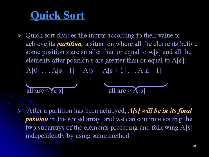
Quick Sort Ø Quick sort divides the inputs according to their value to achieve its partition, a situation where all the elements before some position s are smaller than or equal to A[s] and all the elements after position s are greater than or equal to A[s]: A[0]. . . A[s – 1] A[s + 1]. . . A[n – 1] all are ≤ A[s] Ø all are ≥ A[s] After a partition has been achieved, A[s] will be in its final position in the sorted array, and we can continue sorting the two subarrays of the elements preceding and following A[s] independently by using same method. 35

Quick Sort ALGORITHM Quicksort(A[l. . r]) //Sorts a subarray by quicksort //Input: A subarray A[l. . r] of A[0. . n - 1], defined by its left // and right indices l and r //Output: The subarray A[l. . r] sorted in nondecreasing // order if l < r s Partition(A[l. . r]) //s is a split position Quicksort(A[l. . s - 1]) Quicksort(A[s + 1. . r]) 36

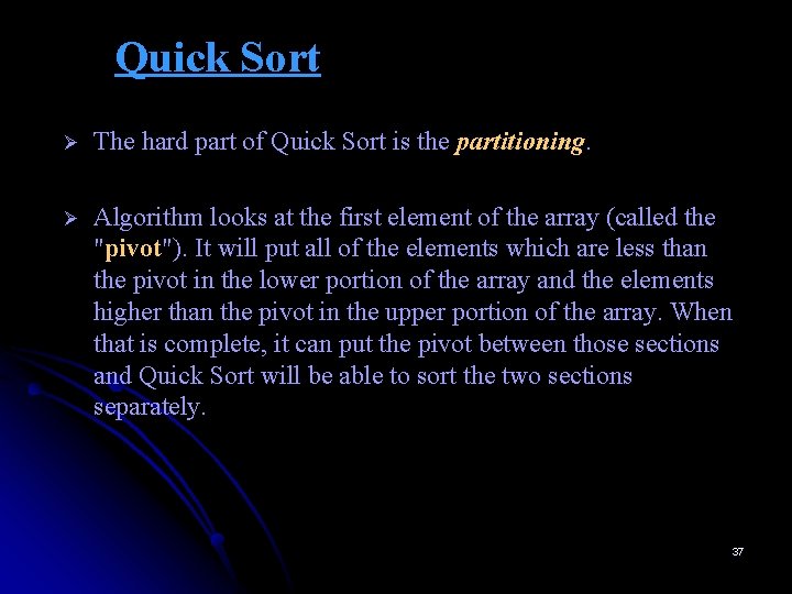
Quick Sort Ø The hard part of Quick Sort is the partitioning. Ø Algorithm looks at the first element of the array (called the "pivot"). It will put all of the elements which are less than the pivot in the lower portion of the array and the elements higher than the pivot in the upper portion of the array. When that is complete, it can put the pivot between those sections and Quick Sort will be able to sort the two sections separately. 37

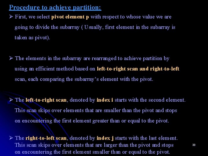
Procedure to achieve partition: Ø First, we select pivot element p with respect to whose value we are going to divide the subarray ( Usually, first element in the subarray is taken as pivot). Ø The elements in the subarray are rearranged to achieve partition by using an efficient method based on left-to-right scan and right-to-left scan, each comparing the subarray’s element with the pivot. Ø The left-to-right scan, denoted by index i starts with the second element. This scan skips over elements that are smaller than the pivot and stops on encountering the first element greater than or equal to the pivot. Ø The right-to-left scan, denoted by index j starts with the last element. This scan skips over elements that are larger than the pivot and stops on encountering the first element smaller than or equal to the pivot. 38

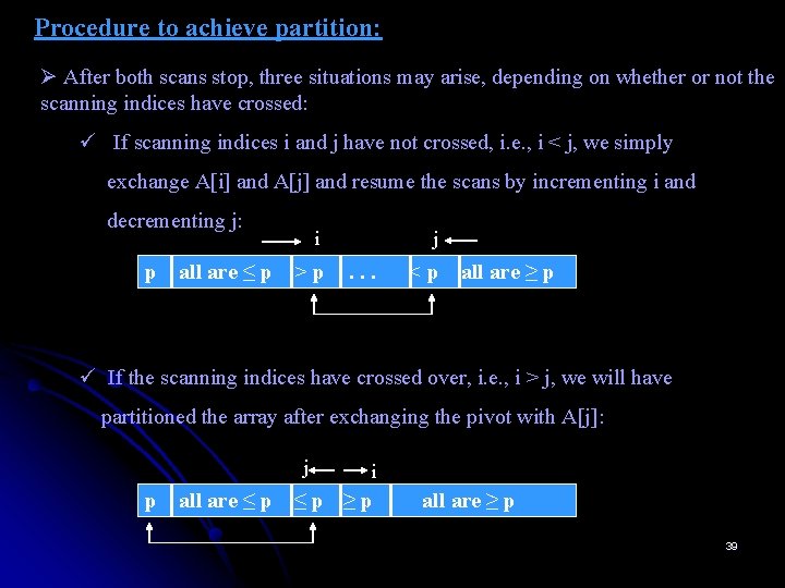
Procedure to achieve partition: Ø After both scans stop, three situations may arise, depending on whether or not the scanning indices have crossed: ü If scanning indices i and j have not crossed, i. e. , i < j, we simply exchange A[i] and A[j] and resume the scans by incrementing i and decrementing j: p all are ≤ p i >p j . . . <p all are ≥ p ü If the scanning indices have crossed over, i. e. , i > j, we will have partitioned the array after exchanging the pivot with A[j]: j p all are ≤ p i ≤p ≥p all are ≥ p 39

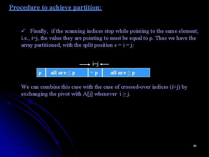
Procedure to achieve partition: ü Finally, if the scanning indices stop while pointing to the same element, i. e. , i=j, the value they are pointing to must be equal to p. Thus we have the array partitioned, with the split position s = i = j: i=j p all are ≤ p =p all are ≥ p We can combine this case with the case of crossed-over indices (i>j) by exchanging the pivot with A[j] whenever i ≥ j. 40

Partition Procedure ALGORITHM Partition(A[l. . r]) //Partitions subarray by using its first element as a pivot //Input: subarray A[l. . r] of A[0. . n - 1], defined by its left and right indices l and r (l< r) //Output: A partition of A[l. . r], with the split position returned as this function’s value p A[l] i l; j r + 1 repeat i i + 1 until A[i] ≥ p repeat j j -1 until A[j ] ≤ p swap(A[i], A[j ]) until i ≥ j swap(A[i], A[j ]) //undo last swap when i ≥ j swap(A[l], A[j ]) 41 return j

1. While A[i] <= A[pivot] ++i Pivot_index = 0 40 20 [0] [1] [2] [3] [4] [5] i 10 80 60 50 7 30 100 [6] [7] [8] j 42

1. While A[i] <= A[pivot] ++i pivot_index = 0 40 20 10 [0] [1] [2] [3] [4] [5] i 80 60 50 7 30 100 [6] [7] [8] j 43

1. While A[i] <= A[pivot] ++i pivot_index = 0 40 20 10 80 [0] [1] [2] [3] [4] [5] i 60 50 7 30 100 [6] [7] [8] j 44

1. While A[i] <= A[pivot] ++i 2. While A[j] > A[pivot] 3. --j pivot_index = 0 40 20 10 80 [0] [1] [2] [3] [4] [5] i 60 50 7 30 100 [6] [7] [8] j 45

1. While A[i] <= A[pivot] ++i 2. While A[j] > A[pivot] 3. --j pivot_index = 0 40 20 10 80 [0] [1] [2] [3] [4] [5] i 60 50 7 30 100 [6] [7] [8] j 46

1. While A[i] <= A[pivot] ++i 2. While A[j] > A[pivot] 3. --j 3. If i < j 4. Swap A[i] and A[j] pivot_index = 0 40 20 10 80 60 50 7 30 100 [0] [1] [2] [3] [4] [5] [6] [7] [8] i j 47

1. While A[i] <= A[pivot] ++i 2. While A[j] > A[pivot] 3. --j 3. If i < j 4. Swap A[i] and A[j] pivot_index = 0 40 20 10 30 60 50 7 80 100 [0] [1] [2] [3] [4] [5] [6] [7] [8] i j 48

1. While A[i] <= A[pivot] ++i 2. While A[j] > A[pivot] 3. --j 3. If i < j 4. Swap A[i] and A[j] 5. 4. While j > i goto step 1 pivot_index = 0 40 20 10 30 60 50 7 80 100 [0] [1] [2] [3] [4] [5] [6] [7] [8] i j 49

1. While A[i] <= A[pivot] ++i 2. While A[j] > A[pivot] 3. --j 3. If i < j 4. Swap A[i] and A[j] 5. 4. While j > i goto step 1 pivot_index = 0 40 20 10 30 60 50 7 80 100 [0] [1] [2] [3] [4] [5] [6] [7] [8] i j 50

1. While A[i] <= A[pivot] ++i 2. While A[j] > A[pivot] 3. --j 3. If i < j 4. Swap A[i] and A[j] 5. 4. While j > i goto step 1 pivot_index = 0 40 20 10 30 60 [0] [1] [2] [3] [4] [5] i 50 7 80 100 [6] [7] [8] j 51

1. While A[i] <= A[pivot] ++i 2. While A[j] > A[pivot] 3. --j 3. If i < j 4. Swap A[i] and A[j] 5. 4. While j > i goto step 1 pivot_index = 0 40 20 10 30 60 [0] [1] [2] [3] [4] [5] i 50 7 80 100 [6] [7] [8] j 52

1. While A[i] <= A[pivot] ++i 2. While A[j] > A[pivot] 3. --j 3. If i < j 4. Swap A[i] and A[j] 5. 4. While j > i goto step 1 pivot_index = 0 40 20 10 30 60 [0] [1] [2] [3] [4] [5] i 50 7 80 100 [6] [7] [8] j 53

1. While A[i] <= A[pivot] ++i 2. While A[j] > A[pivot] 3. --j 3. If i < j 4. Swap A[i] and A[j] 5. 4. While j > i goto step 1 pivot_index = 0 40 20 10 30 60 [0] [1] [2] [3] [4] [5] i 50 7 80 100 [6] [7] [8] j 54

1. While A[i] <= A[pivot] ++i 2. While A[j] > A[pivot] 3. --j 3. If i < j 4. Swap A[i] and A[j] 5. 4. While j > i goto step 1 pivot_index = 0 40 20 10 30 7 [0] [1] [2] [3] [4] [5] i 50 60 80 100 [6] [7] [8] j 55

1. While A[i] <= A[pivot] ++i 2. While A[j] > A[pivot] 3. --j 3. If i < j 4. Swap A[i] and A[j] 5. 4. While j > i goto step 1 pivot_index = 0 40 20 10 30 7 [0] [1] [2] [3] [4] [5] i 50 60 80 100 [6] [7] [8] j 56

1. While A[i] <= A[pivot] ++i 2. While A[j] > A[pivot] 3. --j 3. If i < j 4. Swap A[i] and A[j] 5. 4. While j > i goto step 1 pivot_index = 0 40 20 10 30 7 [0] [1] [2] [3] [4] [5] i 50 60 80 100 [6] [7] [8] j 57

1. While A[i] <= A[pivot] ++i 2. While A[j] > A[pivot] 3. --j 3. If i < j 4. Swap A[i] and A[j] 5. 4. While j > i goto step 1 pivot_index = 0 40 20 10 30 7 50 [0] [1] [2] [3] [4] [5] i 60 80 100 [6] [7] [8] j 58

1. While A[i] <= A[pivot] ++i 2. While A[j] > A[pivot] 3. --j 3. If i < j 4. Swap A[i] and A[j] 5. 4. While j > i goto step 1 pivot_index = 0 40 20 10 30 7 50 [0] [1] [2] [3] [4] [5] i 60 80 100 [6] [7] [8] j 59

1. While A[i] <= A[pivot] ++i 2. While A[j] > A[pivot] 3. --j 3. If i < j 4. Swap A[i] and A[j] 5. 4. While j > i goto step 1 pivot_index = 0 40 20 10 30 7 50 [0] [1] [2] [3] [4] [5] i 60 80 100 [6] [7] [8] j 60

1. While A[i] <= A[pivot] ++i 2. While A[j] > A[pivot] 3. --j 3. If i < j 4. Swap A[i] and A[j] 5. 4. While j > i goto step 1 pivot_index = 0 40 20 10 30 7 [0] [1] [2] [3] [4] [5] j 50 60 80 100 [6] [7] [8] i 61

1. While A[i] <= A[pivot] ++i 2. While A[j] > A[pivot] 3. --j 3. If i < j 4. Swap A[i] and A[j] 5. 4. While j > i goto step 1 pivot_index = 0 40 20 10 30 7 [0] [1] [2] [3] [4] [5] j 50 60 80 100 [6] [7] [8] i 62

1. While A[i] <= A[pivot] ++i 2. While A[j] > A[pivot] 3. --j 3. If i < j 4. Swap A[i] and A[j] 5. 4. While j > i goto step 1 pivot_index = 0 40 20 10 30 7 [0] [1] [2] [3] [4] [5] j 50 60 80 100 [6] [7] [8] i 63

1. While A[i] <= A[pivot] ++i 2. While A[j] > A[pivot] 3. --j 3. If i < j 4. Swap A[i] and A[j] 4. While j > i goto step 1 5. Swap A[j] and A[pivot] pivot_index = 0 40 20 10 30 7 [0] [1] [2] [3] [4] [5] j 50 60 80 100 [6] [7] [8] i 64

1. While A[i] <= A[pivot] ++i 2. While A[j] > A[pivot] 3. --j 3. If i < j 4. Swap A[i] and A[j] 4. While j > i goto step 1 5. Swap A[j] and A[pivot] pivot_index = 4 7 [0] 20 10 30 40 50 [1] [2] [3] [4] [5] j 60 80 100 [6] [7] [8] i 65

Partition Result 7 [0] 20 10 30 40 50 [1] [2] [3] [4] [5] < = A[pivot] 60 80 100 [6] [7] [8] > A[pivot] 66

Recursion: Quicksort Sub-arrays 7 [0] 20 10 30 40 50 [1] [2] [3] [4] [5] < = A[pivot] 60 80 100 [6] [7] [8] > A[pivot] 67

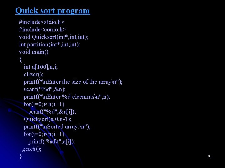
Quick sort program #include<stdio. h> #include<conio. h> void Quicksort(int*, int); int partition(int*, int); void main() { int a[100], n, i; clrscr(); printf("n. Enter the size of the arrayn"); scanf("%d", &n); printf("n. Enter %d eleemntsn", n); for(i=0; i<n; i++) scanf("%d", &a[i]); Quicksort(a, 0, n-1); printf("n. Sorted array: n"); for(i=0; i<n; i++) printf("%dt", a[i]); getch(); } 68

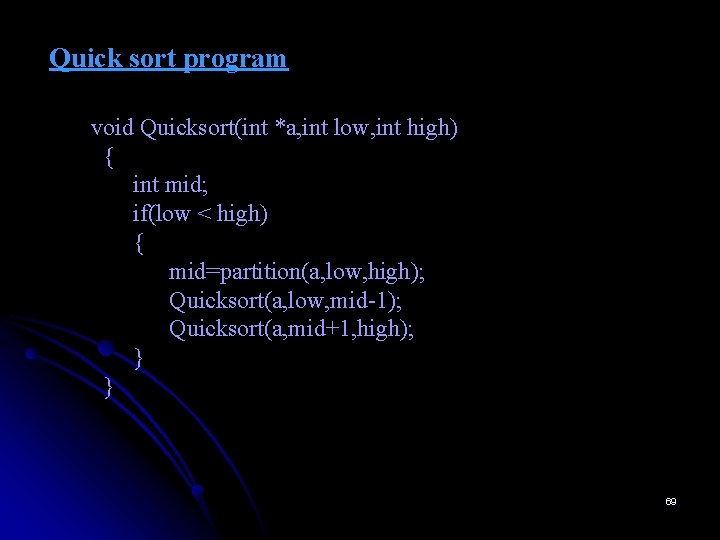
Quick sort program void Quicksort(int *a, int low, int high) { int mid; if(low < high) { mid=partition(a, low, high); Quicksort(a, low, mid-1); Quicksort(a, mid+1, high); } } 69

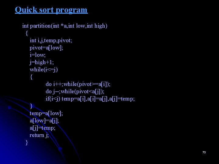
Quick sort program int partition(int *a, int low, int high) { int i, j, temp, pivot; pivot=a[low]; i=low; j=high+1; while(i<=j) { do i++; while(pivot>=a[i]); do j--; while(pivot<a[j]); if(i<j) temp=a[i], a[i]=a[j], a[j]=temp; } temp=a[low]; a[low]=a[j]; a[j]=temp; return j; } 70

a[0] a[1] a[2] a[3] a[4] a[5] a[6] 5 3 1 9 8 2 4 a[7] 7 low = 0, high = 7 mid = 4 low = 0, high = 3 mid = 1 low = 0, high = 0 low = 2, high = 1 low = 5, high = 7 mid = 6 low = 2, high =3 mid = 2 low = 5, high = 5 low = 7, high = 7 low = 3, high = 3 Quicksort Example: Recursion Tree. 71

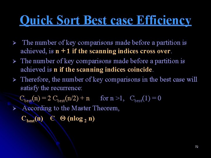
Quick Sort Best case Efficiency Ø Ø The number of key comparisons made before a partition is achieved, is n + 1 if the scanning indices cross over. The number of key comparisons made before a partition is achieved is n if the scanning indices coincide. Therefore, the number of key comparisons in the best case will satisfy the recurrence: Cbest(n) = 2 Cbest(n/2) + n for n >1, Cbest(1) = 0 According to the Master Theorem, Cbest(n) Є Θ (nlog 2 n) 72

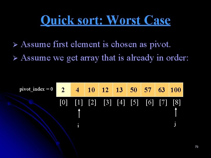
Quick sort: Worst Case Assume first element is chosen as pivot. Ø Assume we get array that is already in order: Ø pivot_index = 0 2 [0] 4 10 12 13 50 [1] [2] [3] [4] [5] i 57 63 100 [6] [7] [8] j 73

1. While A[i] <= A[pivot] ++i 2. While A[j] > A[pivot] 3. --j 3. If i < j 4. Swap A[i] and A[j] 4. While j > i goto step 1 5. Swap A[j] and A[pivot] pivot_index = 0 2 [0] 4 10 12 13 50 [1] [2] [3] [4] [5] i 57 63 100 [6] [7] [8] j 74

1. While A[i] <= A[pivot] ++i 2. While A[j] > A[pivot] 3. --j 3. If i < j 4. Swap A[i] and A[j] 4. While j > i goto step 1 5. Swap A[j] and A[pivot] pivot_index = 0 2 [0] 4 10 12 13 50 [1] [2] [3] [4] [5] i 57 63 100 [6] [7] [8] j 75

1. While A[i] <= A[pivot] ++i 2. While A[j] > A[pivot] 3. --j 3. If i < j 4. Swap A[i] and A[j] 4. While j > i goto step 1 5. Swap A[j] and A[pivot] pivot_index = 0 2 [0] j 4 10 12 13 50 [1] [2] [3] [4] [5] 57 63 100 [6] [7] [8] i 76

1. While A[i] <= A[pivot] ++i 2. While A[j] > A[pivot] 3. --j 3. If i < j 4. Swap A[i] and A[j] 4. While j > i goto step 1 5. Swap A[j] and A[pivot] pivot_index = 0 2 [0] j 4 10 12 13 50 [1] [2] [3] [4] [5] 57 63 100 [6] [7] [8] i 77

1. While A[i] <= A[pivot] ++i 2. While A[j] > A[pivot] 3. --j 3. If i < j 4. Swap A[i] and A[j] 4. While j > i goto step 1 5. Swap A[j] and A[pivot] pivot_index = 0 2 [0] j 4 10 12 13 50 [1] [2] [3] [4] [5] 57 63 100 [6] [7] [8] i 78

1. While A[i] <= A[pivot] ++i 2. While A[j] > A[pivot] 3. --j 3. If i < j 4. Swap A[i] and A[j] 4. While j > i goto step 1 5. Swap A[j] and A[pivot] pivot_index = 0 2 [0] j 4 10 12 13 50 [1] [2] [3] [4] [5] 57 63 100 [6] [7] [8] i 79

1. While A[i] <= A[pivot] ++i 2. While A[j] > A[pivot] 3. --j 3. If i < j 4. Swap A[i] and A[j] 4. While j > i goto step 1 5. Swap A[j] and A[pivot] pivot_index = 0 2 [0] <= data[pivot] 4 10 12 13 50 [1] [2] [3] [4] [5] > data[pivot] 57 63 100 [6] [7] [8] 80

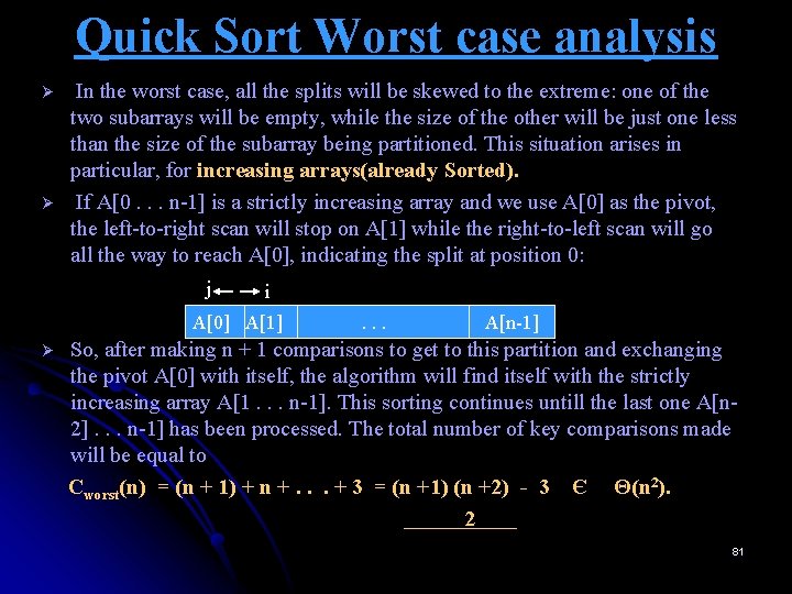
Quick Sort Worst case analysis Ø Ø In the worst case, all the splits will be skewed to the extreme: one of the two subarrays will be empty, while the size of the other will be just one less than the size of the subarray being partitioned. This situation arises in particular, for increasing arrays(already Sorted). If A[0. . . n-1] is a strictly increasing array and we use A[0] as the pivot, the left-to-right scan will stop on A[1] while the right-to-left scan will go all the way to reach A[0], indicating the split at position 0: j i A[0] A[1] Ø . . . A[n-1] So, after making n + 1 comparisons to get to this partition and exchanging the pivot A[0] with itself, the algorithm will find itself with the strictly increasing array A[1. . . n-1]. This sorting continues untill the last one A[n 2]. . . n-1] has been processed. The total number of key comparisons made will be equal to Cworst(n) = (n + 1) + n +. . . + 3 = (n +1) (n +2) - 3 Є Θ(n 2). 2 81

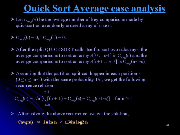
Quick Sort Average case analysis Ø Let Cavg(n) be the average number of key comparisons made by quicksort on a randomly ordered array of size n. Ø Cavg(0) = 0, Cavg(1) = 0. Ø After the split QUICKSORT calls itself to sort two subarrays, the average comparisons to sort an array A[0. . s-1] is Cavg(s) and the average comparisons to sort an array A[s+1. . n-1] is Cavg(n-1 -s). Ø Assuming that the partition split can happen in each position s (0 ≤ s ≤ n-1) with the same probability 1/n, we get the following recurrence relation: n-1 Cavg(n) = 1/n ∑ [(n + 1) + Cavg(s) + Cavg(n-1 -s)] for n > 1 s=0 Ø After solving the above recurrence, we get the solution, Cavg(n) ≈ 2 n ln n ≈ 1. 38 n log 2 n 82

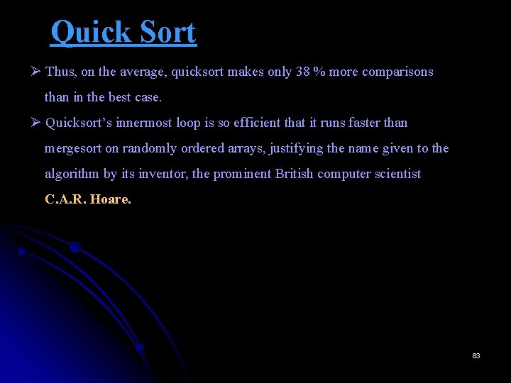
Quick Sort Ø Thus, on the average, quicksort makes only 38 % more comparisons than in the best case. Ø Quicksort’s innermost loop is so efficient that it runs faster than mergesort on randomly ordered arrays, justifying the name given to the algorithm by its inventor, the prominent British computer scientist C. A. R. Hoare. 83

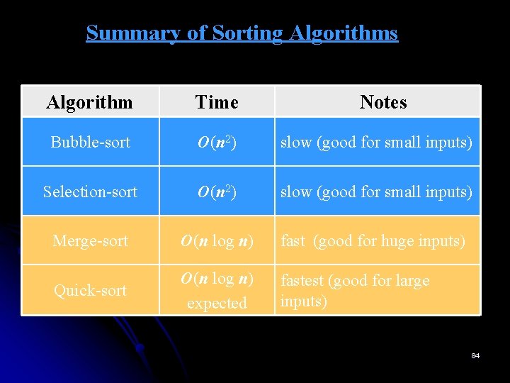
Summary of Sorting Algorithms Algorithm Time Notes Bubble-sort O(n 2) slow (good for small inputs) Selection-sort O(n 2) slow (good for small inputs) Merge-sort O(n log n) fast (good for huge inputs) Quick-sort O(n log n) expected fastest (good for large inputs) 84

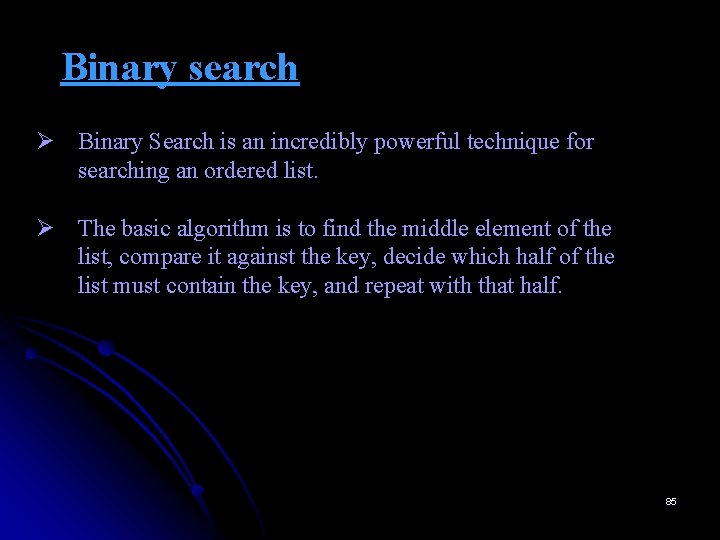
Binary search Ø Binary Search is an incredibly powerful technique for searching an ordered list. Ø The basic algorithm is to find the middle element of the list, compare it against the key, decide which half of the list must contain the key, and repeat with that half. 85

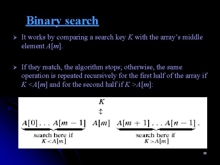
Binary search Ø It works by comparing a search key K with the array’s middle element A[m]. Ø If they match, the algorithm stops; otherwise, the same operation is repeated recursively for the first half of the array if K <A[m] and for the second half if K >A[m]: 86

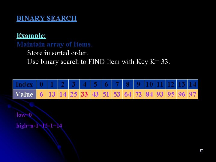
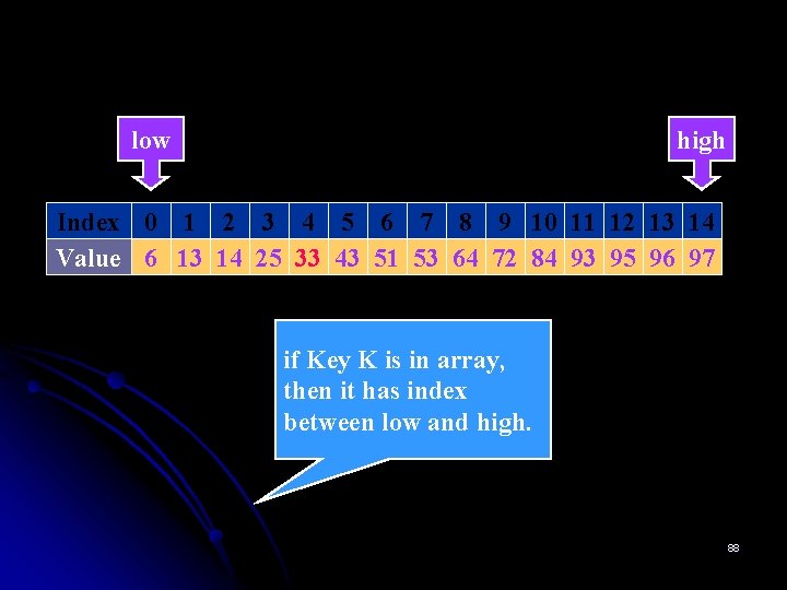
BINARY SEARCH Example: Maintain array of Items. Store in sorted order. Use binary search to FIND Item with Key K= 33. Index 0 1 2 3 4 5 6 7 8 9 10 11 12 13 14 Value 6 13 14 25 33 43 51 53 64 72 84 93 95 96 97 low=0 high=n-1=15 -1=14 87

low high Index 0 1 2 3 4 5 6 7 8 9 10 11 12 13 14 Value 6 13 14 25 33 43 51 53 64 72 84 93 95 96 97 if Key K is in array, then it has index between low and high. 88

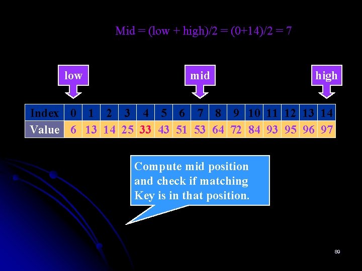
Mid = (low + high)/2 = (0+14)/2 = 7 low mid high Index 0 1 2 3 4 5 6 7 8 9 10 11 12 13 14 Value 6 13 14 25 33 43 51 53 64 72 84 93 95 96 97 Compute mid position and check if matching Key is in that position. 89

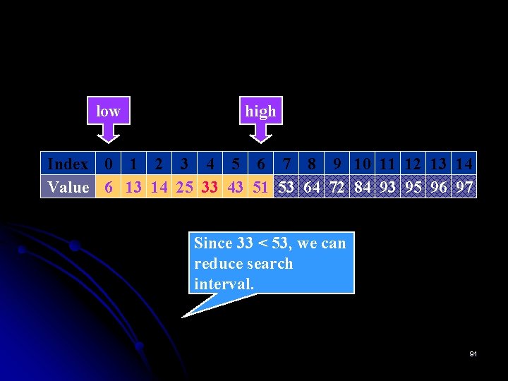
if (Key < a[mid]) high=mid-1 low mid high Index 0 1 2 3 4 5 6 7 8 9 10 11 12 13 14 Value 6 13 14 25 33 43 51 53 64 72 84 93 95 96 97 Since 33 < 53, we can reduce search interval. 90

low high Index 0 1 2 3 4 5 6 7 8 9 10 11 12 13 14 Value 6 13 14 25 33 43 51 53 64 72 84 93 95 96 97 Since 33 < 53, we can reduce search interval. 91

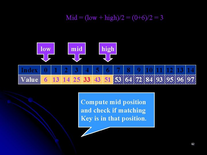
Mid = (low + high)/2 = (0+6)/2 = 3 low mid high Index 0 1 2 3 4 5 6 7 8 9 10 11 12 13 14 Value 6 13 14 25 33 43 51 53 64 72 84 93 95 96 97 Compute mid position and check if matching Key is in that position. 92

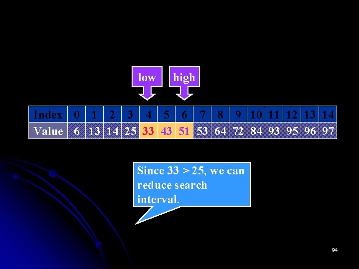
if (Key > a[mid]) low=mid+1 low mid high Index 0 1 2 3 4 5 6 7 8 9 10 11 12 13 14 Value 6 13 14 25 33 43 51 53 64 72 84 93 95 96 97 Since 33 > 25, we can reduce search interval. 93

low high Index 0 1 2 3 4 5 6 7 8 9 10 11 12 13 14 Value 6 13 14 25 33 43 51 53 64 72 84 93 95 96 97 Since 33 > 25, we can reduce search interval. 94

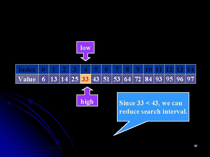
Mid = (low + high)/2 = (4+6)/2 = 5 If (key < a[mid]) low high=mid-1 high Index 0 1 2 3 4 5 6 7 8 9 10 11 12 13 14 Value 6 13 14 25 33 43 51 53 64 72 84 93 95 96 97 mid Compute mid position and check if matching Key is in that position. 95

low Index 0 1 2 3 4 5 6 7 8 9 10 11 12 13 14 Value 6 13 14 25 33 43 51 53 64 72 84 93 95 96 97 high Since 33 < 43, we can reduce search interval. 96

Mid = (low + high)/2 = (4+4)/2 = 4 If (key == a[mid]) return mid low Index 0 1 2 3 4 5 6 7 8 9 10 11 12 13 14 Value 6 13 14 25 33 43 51 53 64 72 84 93 95 96 97 high Matching Key found. Return index 4. 97

Binary Search Algorithm ALGORITHM Binary. Search(A[0. . . n-1], K) //Implements nonrecursive binary search //Input: An array A[0. . . n-1] sorted in ascending order // and a search key K //Output: An index of the array’s element that is equal // to K or -1 if there is no such element l ← 0; r ← n -1 while l ≤ r do m ← (l + r)/2 if K = A[m] return m else if K < A[m] r ← m – 1 else l ← m + 1 return -1 98

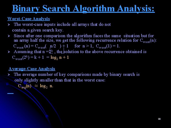
Binary Search Algorithm Analysis: Worst-Case Analysis Ø The worst-case inputs include all arrays that do not contain a given search key. Ø Since after one comparison the algorithm faces the same situation but for an array half the size, we get the following recurrence relation for Cworst(n): Cworst (n) = Cworst( n/2 ) + 1 for n > 1, Cworst(1) = 1. Ø Assuming that n =2 k , the solution to the above recurrence obtained is Cworst(2 k) = k + 1 = log 2 n + 1 Average-Case Analysis Ø The average number of key comparisons made by binary search is only slightly smaller than that in the worst case: Cavg(n) ≈ log 2 n. 99

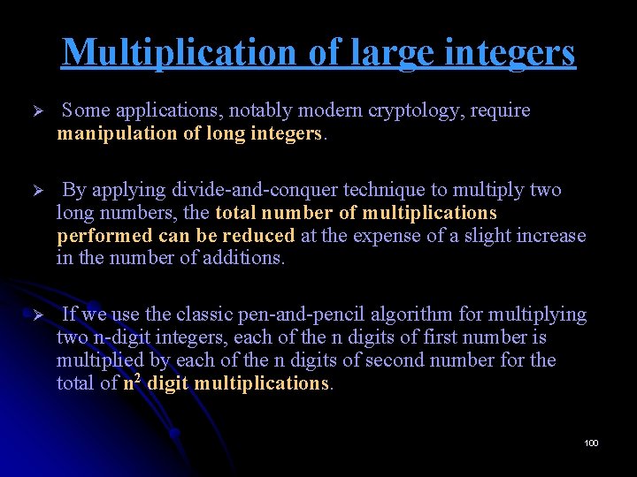
Multiplication of large integers Ø Some applications, notably modern cryptology, require manipulation of long integers. Ø By applying divide-and-conquer technique to multiply two long numbers, the total number of multiplications performed can be reduced at the expense of a slight increase in the number of additions. Ø If we use the classic pen-and-pencil algorithm for multiplying two n-digit integers, each of the n digits of first number is multiplied by each of the n digits of second number for the total of n 2 digit multiplications. 100

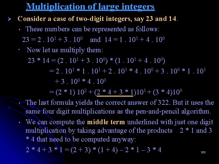
Multiplication of large integers Ø Consider a case of two-digit integers, say 23 and 14. • These numbers can be represented as follows: 23 = 2. 101 + 3. 100 and 14 = 1. 101 + 4. 100 • Now let us multiply them: 23 * 14 = (2. 101 + 3. 100) * (1. 101 + 4. 100) = 2. 101 * 1. 101 + 2. 101 * 4. 100 + 3. 100 * 1. 101 + 3. 100 * 4. 100 = (2 * 1) 102 + (2 * 4 + 3 * 1)101 + (3 * 4)100 • The last formula yields the correct answer of 322. But it uses the same four digit multiplications as the pen-and-pencil algorithm. • We can compute the middle term underlined with just one digit multiplication by taking advantage of the products 2 * 1 and 3 * 4 that need to be computed anyway: 2 * 4 + 3 * 1 = (2 + 3) * (1 + 4) – 2 * 1 – 3 * 4 101

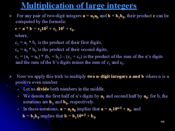
Multiplication of large integers Ø For any pair of two-digit integers a = a 1 a 0 and b = b 1 b 0, their product c can be computed by the formula: c = a * b = c 2102 + c 1 101 + c 0 , where, c 2 = a 1 * b 1 is the product of their first digits, c 0 = a 0 * b 0 is the product of their second digits, c 1 = (a 1 + a 0) * (b 1 + b 0) – (c 2 + c 0) is the product of the sum of the a’s digits and the sum of the b’s digits minus the sum of c 2 and c 0. Ø Now we apply this trick to multiply two n-digit integers a and b where n is a positive even number. • Let us divide both numbers in the middle. • We denote the first half of a’s digits by a 1 and second half by a 0; for b, the notations are b 1 and b 0, respectively. • In these notations, a = a 1 a 0 implies that a = a 110 n/2 + a 0, and b = b 1 b 0 implies that b = b 110 n/2 + b 0. 102

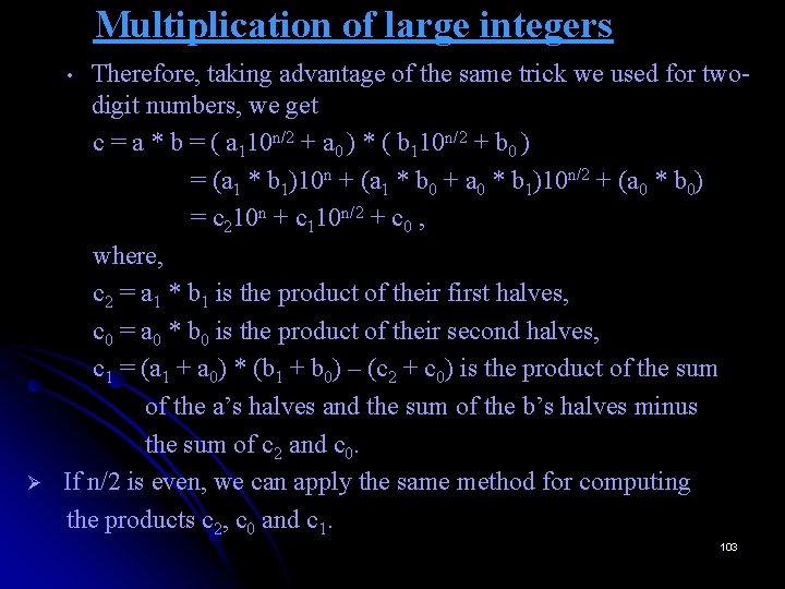
Multiplication of large integers Therefore, taking advantage of the same trick we used for twodigit numbers, we get c = a * b = ( a 110 n/2 + a 0 ) * ( b 110 n/2 + b 0 ) = (a 1 * b 1)10 n + (a 1 * b 0 + a 0 * b 1)10 n/2 + (a 0 * b 0) = c 210 n + c 110 n/2 + c 0 , where, c 2 = a 1 * b 1 is the product of their first halves, c 0 = a 0 * b 0 is the product of their second halves, c 1 = (a 1 + a 0) * (b 1 + b 0) – (c 2 + c 0) is the product of the sum of the a’s halves and the sum of the b’s halves minus the sum of c 2 and c 0. If n/2 is even, we can apply the same method for computing the products c 2, c 0 and c 1. • Ø 103

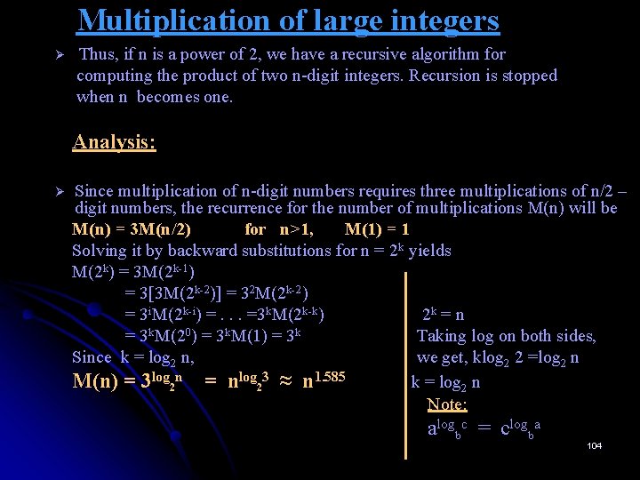
Multiplication of large integers Ø Thus, if n is a power of 2, we have a recursive algorithm for computing the product of two n-digit integers. Recursion is stopped when n becomes one. Analysis: Ø Since multiplication of n-digit numbers requires three multiplications of n/2 – digit numbers, the recurrence for the number of multiplications M(n) will be M(n) = 3 M(n/2) for n>1, M(1) = 1 Solving it by backward substitutions for n = 2 k yields M(2 k) = 3 M(2 k-1) = 3[3 M(2 k-2)] = 32 M(2 k-2) = 3 i. M(2 k-i) =. . . =3 k. M(2 k-k) 2 k = n = 3 k. M(20) = 3 k. M(1) = 3 k Taking log on both sides, Since k = log 2 n, we get, klog 2 2 =log 2 n M(n) = 3 log 2 n = nlog 23 ≈ n 1. 585 k = log 2 n Note: alogbc = clogba 104

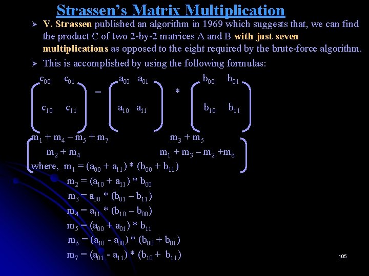
Strassen’s Matrix Multiplication V. Strassen published an algorithm in 1969 which suggests that, we can find the product C of two 2 -by-2 matrices A and B with just seven multiplications as opposed to the eight required by the brute-force algorithm. Ø This is accomplished by using the following formulas: c 00 c 01 a 00 a 01 b 00 b 01 = * c 10 c 11 a 10 a 11 b 10 b 11 Ø m 1 + m 4 – m 5 + m 7 m 3 + m 5 m 2 + m 4 m 1 + m 3 – m 2 +m 6 where, m 1 = (a 00 + a 11) * (b 00 + b 11) m 2 = (a 10 + a 11) * b 00 m 3 = a 00 * (b 01 – b 11) m 4 = a 11 * (b 10 – b 00) m 5 = (a 00 + a 01) * b 11 m 6 = (a 10 - a 00) * (b 00 + b 01) m 7 = (a 01 - a 11) * (b 10 + b 11) 105

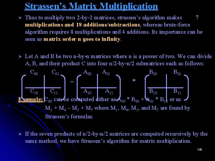
Strassen’s Matrix Multiplication Ø Thus to multiply two 2 -by-2 matrices, strassen’s algorithm makes 7 multiplications and 18 additions/subtractions, whereas brute-force algorithm requires 8 multiplications and 4 additions. Its importance can be seen as matrix order n goes to infinity. Ø Let A and B be two n-by-n matrices where n is a power of two. We can divide A, B, and their product C into four n/2 -by-n/2 submatrices each as follows: C 00 C 01 A 00 A 01 B 00 B 01 = * C 10 C 11 A 10 A 11 B 10 B 11 Example: C 00 can be computed either as A 00 * B 00 + A 01 * B 10 or as M 1 + M 4 – M 5 + M 7 where M 1, M 4, M 5, and M 7 are found by Strassen’s formulas. Ø If the seven products of n/2 -by-n/2 matrices are computed recursively by the same method, we have Strassen’s algorithm for matrix multiplication. 106

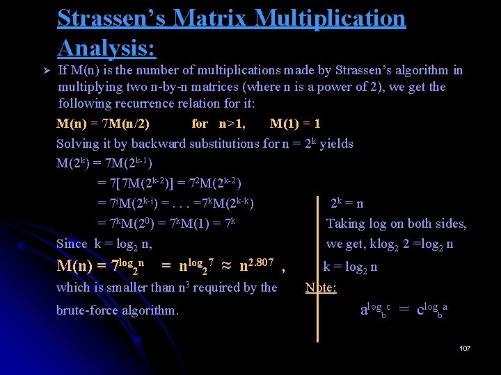
Strassen’s Matrix Multiplication Analysis: Ø If M(n) is the number of multiplications made by Strassen’s algorithm in multiplying two n-by-n matrices (where n is a power of 2), we get the following recurrence relation for it: M(n) = 7 M(n/2) for n>1, M(1) = 1 Solving it by backward substitutions for n = 2 k yields M(2 k) = 7 M(2 k-1) = 7[7 M(2 k-2)] = 72 M(2 k-2) = 7 i. M(2 k-i) =. . . =7 k. M(2 k-k) 2 k = n = 7 k. M(20) = 7 k. M(1) = 7 k Taking log on both sides, Since k = log 2 n, we get, klog 2 2 =log 2 n M(n) = 7 log 2 n = nlog 27 ≈ n 2. 807 , which is smaller than n 3 required by the brute-force algorithm. k = log 2 n Note: alogbc = clogba 107

End of Chapter 4 108