Recursive sorting algorithms Oh no not again sorting
![Mergesort function template <class item> void mergesort (item data[ ], size_t n) { size_t Mergesort function template <class item> void mergesort (item data[ ], size_t n) { size_t](https://slidetodoc.com/presentation_image/58585cd4754de55562774073b3dd014f/image-8.jpg)
![Code for merge template <class item> void merge (item data[ ], size_t n 1, Code for merge template <class item> void merge (item data[ ], size_t n 1,](https://slidetodoc.com/presentation_image/58585cd4754de55562774073b3dd014f/image-17.jpg)

![Code for Quicksort template <class item> void quicksort (item data[ ], size_t n) { Code for Quicksort template <class item> void quicksort (item data[ ], size_t n) {](https://slidetodoc.com/presentation_image/58585cd4754de55562774073b3dd014f/image-28.jpg)

- Slides: 35

Recursive sorting algorithms Oh no, not again! sorting 2 1

Recursive sorting algorithms • Recursive algorithms are considerably more efficient than quadratic algorithms • The downside is they are harder to comprehend and thus harder to code • Two examples of recursive algorithms that use a divide and conquer paradigm are Mergesort and Quicksorting 2 2

Divide and Conquer sorting paradigm • Divide elements to be sorting into two (nearly) equal groups • Sort each of these smaller groups (by recursive calls) • Combine the two sorted groups into one large sorted list sorting 2 3

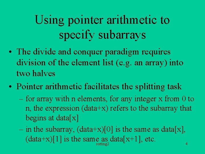
Using pointer arithmetic to specify subarrays • The divide and conquer paradigm requires division of the element list (e. g. an array) into two halves • Pointer arithmetic facilitates the splitting task – for array with n elements, for any integer x from 0 to n, the expression (data+x) refers to the subarray that begins at data[x] – in the subarray, (data+x)[0] is the same as data[x], (data+x)[1] is the samesorting 2 as data[x+1], etc. 4

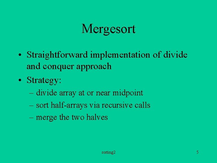
Mergesort • Straightforward implementation of divide and conquer approach • Strategy: – divide array at or near midpoint – sort half-arrays via recursive calls – merge the two halves sorting 2 5

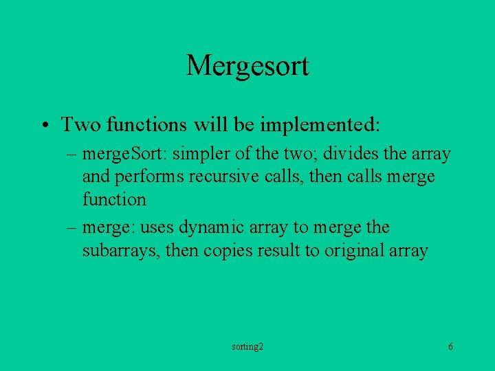
Mergesort • Two functions will be implemented: – merge. Sort: simpler of the two; divides the array and performs recursive calls, then calls merge function – merge: uses dynamic array to merge the subarrays, then copies result to original array sorting 2 6

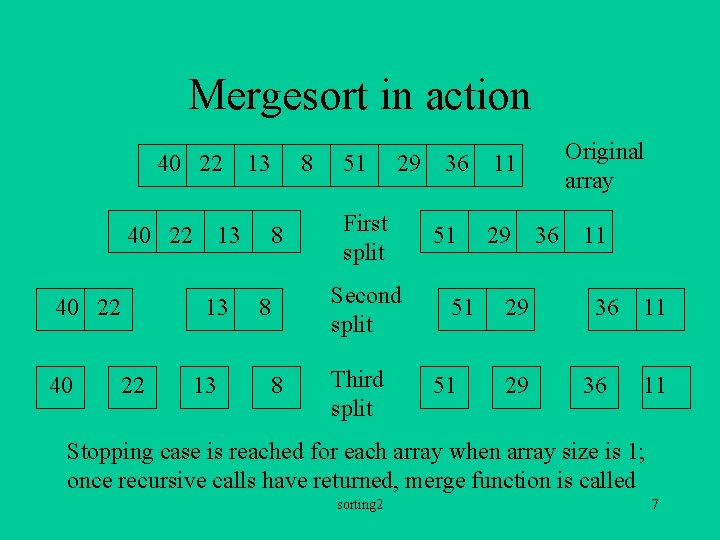
Mergesort in action 40 22 40 8 13 13 22 13 13 8 51 29 First split Second split 8 8 Third split 36 51 51 51 11 29 36 29 29 Original array 11 36 36 11 11 Stopping case is reached for each array when array size is 1; once recursive calls have returned, merge function is called sorting 2 7
![Mergesort function template class item void mergesort item data sizet n sizet Mergesort function template <class item> void mergesort (item data[ ], size_t n) { size_t](https://slidetodoc.com/presentation_image/58585cd4754de55562774073b3dd014f/image-8.jpg)
Mergesort function template <class item> void mergesort (item data[ ], size_t n) { size_t n 1, n 2; // sizes of the two subarrays if (n > 1) { n 1 = n / 2; n 2 = n - n 1; mergesort (data, n 1); mergesort ((data + n 1), n 2); merge (data, n 1, n 2); } } sorting 2 8

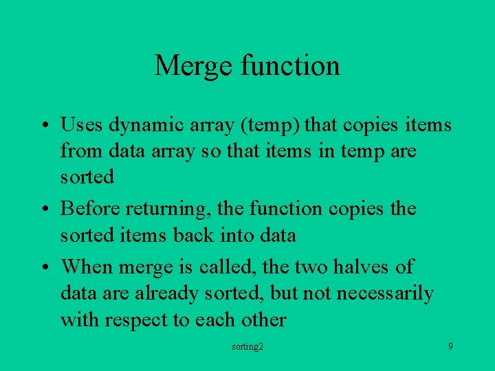
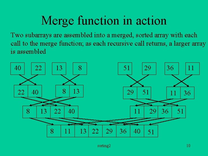
Merge function • Uses dynamic array (temp) that copies items from data array so that items in temp are sorted • Before returning, the function copies the sorted items back into data • When merge is called, the two halves of data are already sorted, but not necessarily with respect to each other sorting 2 9

Merge function in action Two subarrays are assembled into a merged, sorted array with each call to the merge function; as each recursive call returns, a larger array is assembled 40 22 13 8 22 40 8 8 13 22 8 51 13 29 40 11 29 13 22 29 sorting 2 36 36 51 11 11 29 36 40 51 11 36 51 10

How merge works • As shown in the previous example, the first call to merge deals with several half-arrays of size 1; merge creates a temporary array large enough to hold all elements of both halves, and arranges these elements in order • Each subsequent call performs a similar operation on progressively larger, presorted half-arrays sorting 2 11

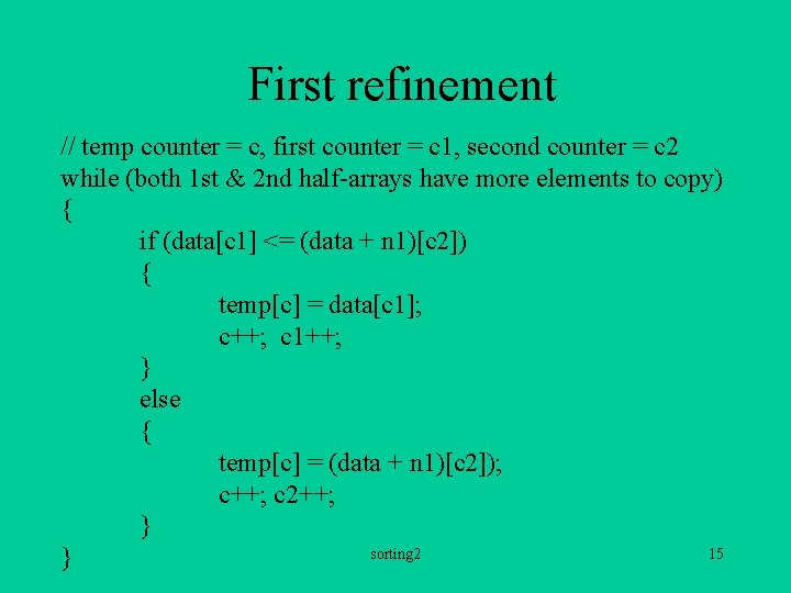
How merge works • Each instance of merge contains the dynamic array temp, and three counters: one that keeps track of the total number of elements copied to temp, and one each to track the number of elements copied from each half-array • The counters are used as indexes to the three arrays: the first half-array (data), the second half-array (data + n 1) and the dynamic array (temp) sorting 2 12

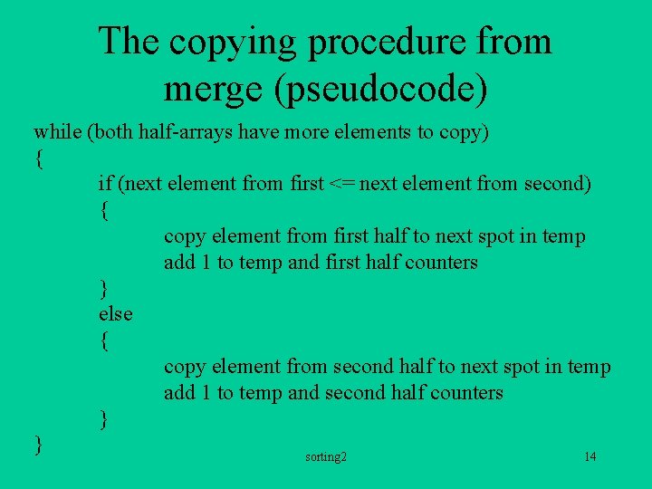
How merge works • Elements are copied one-by-one from the two half -arrays, with the smallest elements from both copied first • When all elements of either half-array have been copied, the remaining elements of the other halfarray are copied to the end of temp • Because the half-arrays are pre-sorted, these “leftover” elements will be the largest values in each half-array sorting 2 13

The copying procedure from merge (pseudocode) while (both half-arrays have more elements to copy) { if (next element from first <= next element from second) { copy element from first half to next spot in temp add 1 to temp and first half counters } else { copy element from second half to next spot in temp add 1 to temp and second half counters } } sorting 2 14

First refinement // temp counter = c, first counter = c 1, second counter = c 2 while (both 1 st & 2 nd half-arrays have more elements to copy) { if (data[c 1] <= (data + n 1)[c 2]) { temp[c] = data[c 1]; c++; c 1++; } else { temp[c] = (data + n 1)[c 2]); c++; c 2++; } sorting 2 15 }

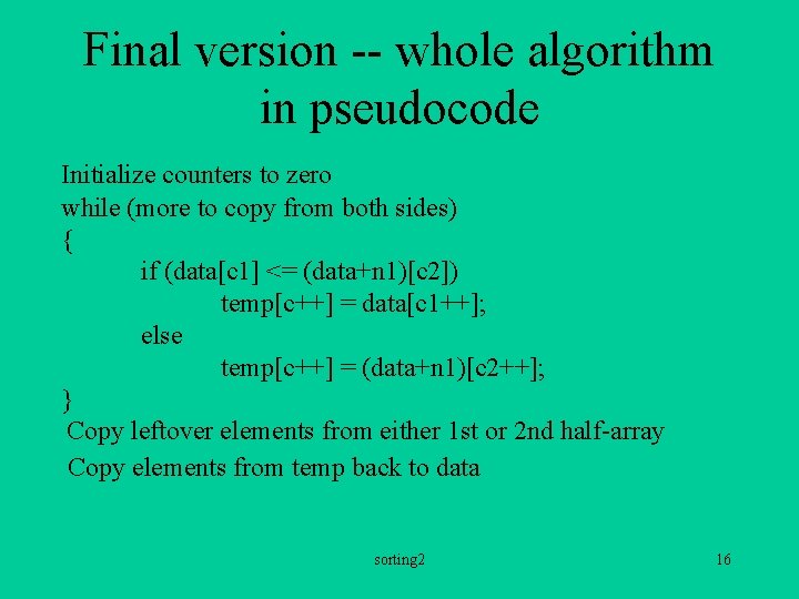
Final version -- whole algorithm in pseudocode Initialize counters to zero while (more to copy from both sides) { if (data[c 1] <= (data+n 1)[c 2]) temp[c++] = data[c 1++]; else temp[c++] = (data+n 1)[c 2++]; } Copy leftover elements from either 1 st or 2 nd half-array Copy elements from temp back to data sorting 2 16
![Code for merge template class item void merge item data sizet n 1 Code for merge template <class item> void merge (item data[ ], size_t n 1,](https://slidetodoc.com/presentation_image/58585cd4754de55562774073b3dd014f/image-17.jpg)
Code for merge template <class item> void merge (item data[ ], size_t n 1, size_t n 2) { item* temp; size_t c=0, c 1=0, c 2=0; temp = new item[n 1 + n 2]; while ((c 1 < n 1) && (c 2 < n 2)) { if (data[c 1] < (data + n 1)[c 2]) temp[c++] = data[c 1++]; else temp[c++] = (data + n 1)[c 2++]; } sorting 2 17

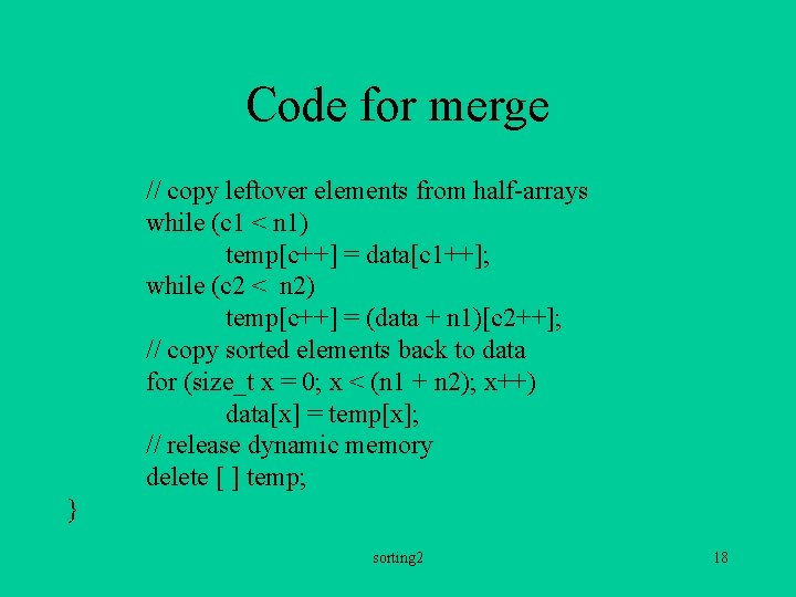
Code for merge // copy leftover elements from half-arrays while (c 1 < n 1) temp[c++] = data[c 1++]; while (c 2 < n 2) temp[c++] = (data + n 1)[c 2++]; // copy sorted elements back to data for (size_t x = 0; x < (n 1 + n 2); x++) data[x] = temp[x]; // release dynamic memory delete [ ] temp; } sorting 2 18

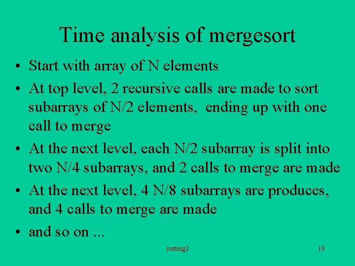
Time analysis of mergesort • Start with array of N elements • At top level, 2 recursive calls are made to sort subarrays of N/2 elements, ending up with one call to merge • At the next level, each N/2 subarray is split into two N/4 subarrays, and 2 calls to merge are made • At the next level, 4 N/8 subarrays are produces, and 4 calls to merge are made • and so on. . . sorting 2 19

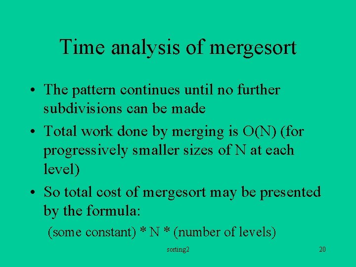
Time analysis of mergesort • The pattern continues until no further subdivisions can be made • Total work done by merging is O(N) (for progressively smaller sizes of N at each level) • So total cost of mergesort may be presented by the formula: (some constant) * N * (number of levels) sorting 2 20

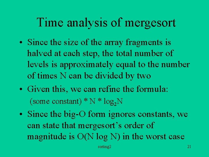
Time analysis of mergesort • Since the size of the array fragments is halved at each step, the total number of levels is approximately equal to the number of times N can be divided by two • Given this, we can refine the formula: (some constant) * N * log 2 N • Since the big-O form ignores constants, we can state that mergesort’s order of magnitude is O(N log N) in the worst case sorting 2 21

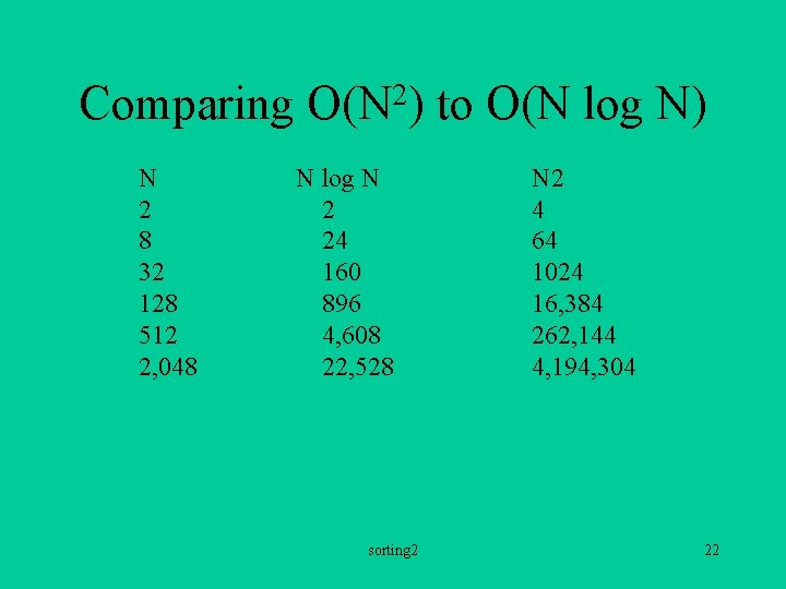
Comparing N 2 8 32 128 512 2, 048 2 O(N ) N log N 2 24 160 896 4, 608 22, 528 sorting 2 to O(N log N) N 2 4 64 1024 16, 384 262, 144 4, 194, 304 22

Application of Mergesort • Although more efficient than a quadratic algorithm, mergesort is not the best choice for sorting arrays because of the need for a temporary dynamic array in the merge step • The algorithm is often used for sorting files • With each call to mergesort, the file is split into smaller and smaller pieces; once a piece is small enough to fit into an array, a more efficient sorting algorithm can be applied to it sorting 2 23

Quicksort • Similar to Mergesort in its use of divide and conquer paradigm • In Mergesort, the “divide” part was trivial; the array was simply halved. The complicated part was the merge • In Quicksort, the opposite is true; combining the sorted pieces is trivial, but Quicksort uses a sophisticated division algorithm sorting 2 24

Quicksort • Select an element that belongs in the middle of the array (called the pivot), and place it at the midpoint • Place all values less than the pivot before the pivot, and all elements greater than the pivot after the pivot sorting 2 25

Quicksort • At this point, the array is not sorted, but it is closer to being sorted -- the pivot is in the correct position, and all other elements are in the correct array segment • Because the two segments are placed correctly with respect to the pivot, we know that no element needs to be moved from one to the other sorting 2 26

Quicksort • Since we now have the two segments to sort, can perform recursive calls on these segments • Choice of pivot element important to efficiency of algorithm; unfortunately, there is no obvious way to do this • For now, we will arbitrarily pick a value to use as pivot sorting 2 27
![Code for Quicksort template class item void quicksort item data sizet n Code for Quicksort template <class item> void quicksort (item data[ ], size_t n) {](https://slidetodoc.com/presentation_image/58585cd4754de55562774073b3dd014f/image-28.jpg)
Code for Quicksort template <class item> void quicksort (item data[ ], size_t n) { size_t pivot_index; // array index of pivot size_t n 1, n 2; // number of elements before & after pivot if (n > 1) { partition (data, n, pivot_index); n 1 = pivot_index; n 2 = n - n 1 - 1; quicksort (data, n 1); quicksort ((data+pivot_index+1), n 2); } } sorting 2 28

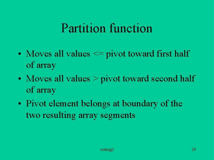
Partition function • Moves all values <= pivot toward first half of array • Moves all values > pivot toward second half of array • Pivot element belongs at boundary of the two resulting array segments sorting 2 29

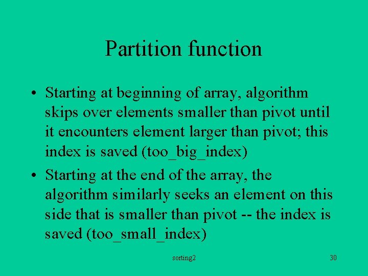
Partition function • Starting at beginning of array, algorithm skips over elements smaller than pivot until it encounters element larger than pivot; this index is saved (too_big_index) • Starting at the end of the array, the algorithm similarly seeks an element on this side that is smaller than pivot -- the index is saved (too_small_index) sorting 2 30

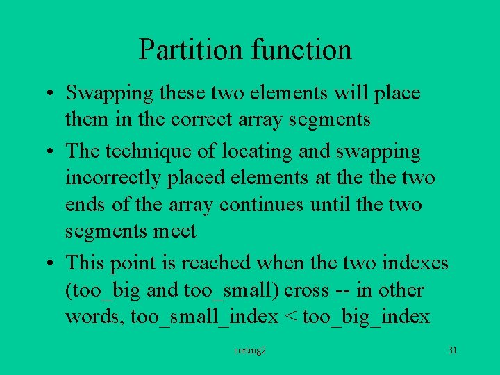
Partition function • Swapping these two elements will place them in the correct array segments • The technique of locating and swapping incorrectly placed elements at the two ends of the array continues until the two segments meet • This point is reached when the two indexes (too_big and too_small) cross -- in other words, too_small_index < too_big_index sorting 2 31

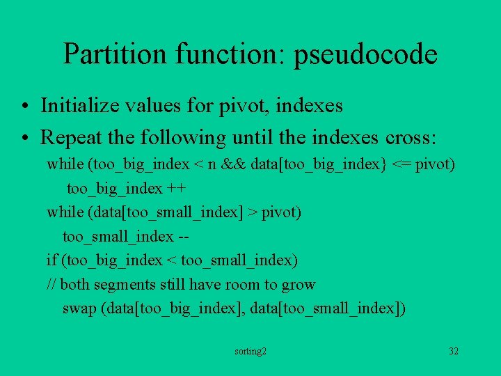
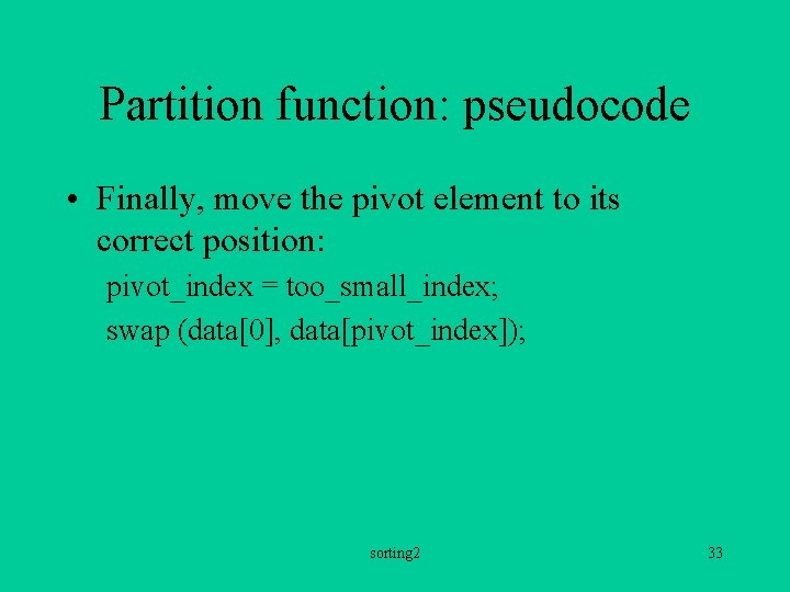
Partition function: pseudocode • Initialize values for pivot, indexes • Repeat the following until the indexes cross: while (too_big_index < n && data[too_big_index} <= pivot) too_big_index ++ while (data[too_small_index] > pivot) too_small_index -if (too_big_index < too_small_index) // both segments still have room to grow swap (data[too_big_index], data[too_small_index]) sorting 2 32

Partition function: pseudocode • Finally, move the pivot element to its correct position: pivot_index = too_small_index; swap (data[0], data[pivot_index]); sorting 2 33

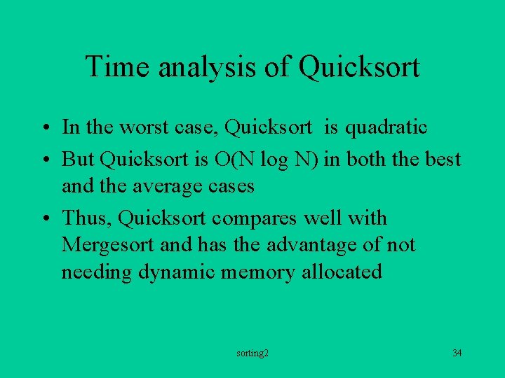
Time analysis of Quicksort • In the worst case, Quicksort is quadratic • But Quicksort is O(N log N) in both the best and the average cases • Thus, Quicksort compares well with Mergesort and has the advantage of not needing dynamic memory allocated sorting 2 34

Choosing a good pivot element • The worst case of Quicksort comes about if the element chosen for pivot is at either extreme - in other words, the smallest or largest element -- this will occur if the array is already sorted! • To decrease the likelihood of this occurring, pick three values at random from the array, and choose the middle of the three as the pivot sorting 2 35