Algorithms Chapter 3 Chapter Summary Algorithms Example Algorithms

Algorithms Chapter 3

Chapter Summary �Algorithms �Example Algorithms �Algorithmic Paradigms �Growth of Functions �Big-O and other Notation �Complexity of Algorithms

Algorithms Section 3. 1

Section Summary �Properties of Algorithms �Algorithms for Searching and Sorting �Greedy Algorithms

Algorithms Definition: An algorithm is a finite set of precise instructions for performing a computation or for solving a problem. Example: Describe an algorithm for finding the maximum value in a finite sequence of integers. Solution: Perform the following steps: 1. 2. � 3. 4. Set the temporary maximum equal to the first integer in the sequence. Compare the next integer in the sequence to the temporary maximum. If it is larger than the temporary maximum, set the temporary maximum equal to this integer. Repeat the previous step if there are more integers. If not, stop. When the algorithm terminates, the temporary maximum is the largest integer in the sequence.

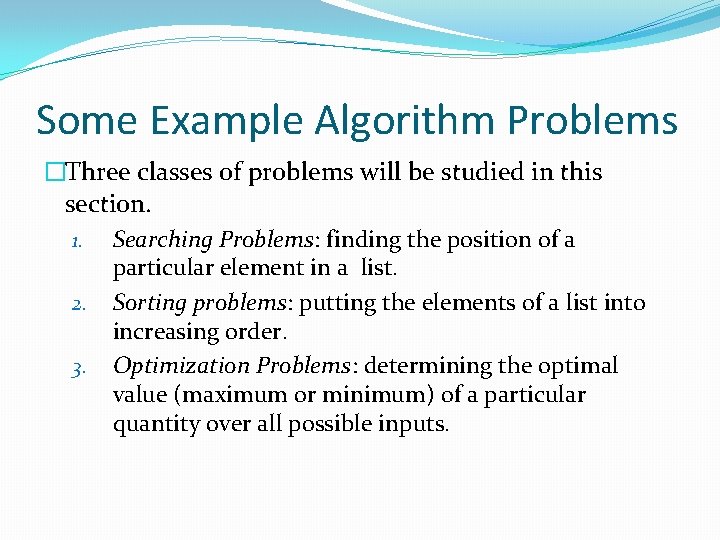
Some Example Algorithm Problems �Three classes of problems will be studied in this section. 1. Searching Problems: finding the position of a particular element in a list. 2. Sorting problems: putting the elements of a list into increasing order. 3. Optimization Problems: determining the optimal value (maximum or minimum) of a particular quantity over all possible inputs.

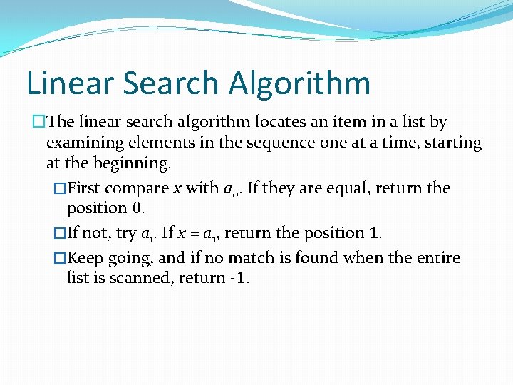
Linear Search Algorithm �The linear search algorithm locates an item in a list by examining elements in the sequence one at a time, starting at the beginning. �First compare x with a 0. If they are equal, return the position 0. �If not, try a 1. If x = a 1, return the position 1. �Keep going, and if no match is found when the entire list is scanned, return -1.

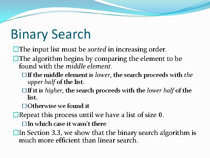
Binary Search �The input list must be sorted in increasing order. �The algorithm begins by comparing the element to be found with the middle element. �If the middle element is lower, the search proceeds with the upper half of the list. �If it is higher, the search proceeds with the lower half of the list. �Otherwise we found it �Repeat this process until we have a list of size 0. �In which case it wasn’t there �In Section 3. 3, we show that the binary search algorithm is much more efficient than linear search.

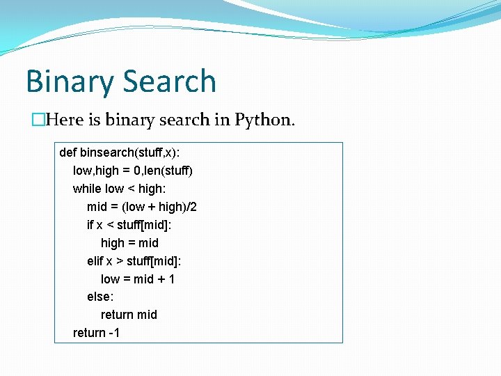
Binary Search �Here is binary search in Python. def binsearch(stuff, x): low, high = 0, len(stuff) while low < high: mid = (low + high)/2 if x < stuff[mid]: high = mid elif x > stuff[mid]: low = mid + 1 else: return mid return -1

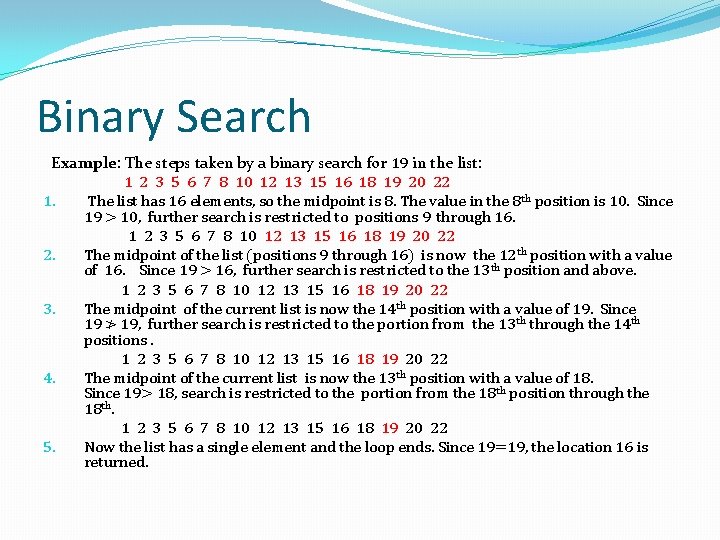
Binary Search Example: The steps taken by a binary search for 19 in the list: 1 2 3 5 6 7 8 10 12 13 15 16 18 19 20 22 1. The list has 16 elements, so the midpoint is 8. The value in the 8 th position is 10. Since 19 > 10, further search is restricted to positions 9 through 16. 1 2 3 5 6 7 8 10 12 13 15 16 18 19 20 22 2. The midpoint of the list (positions 9 through 16) is now the 12 th position with a value of 16. Since 19 > 16, further search is restricted to the 13 th position and above. 1 2 3 5 6 7 8 10 12 13 15 16 18 19 20 22 3. The midpoint of the current list is now the 14 th position with a value of 19. Since 19 ≯ 19, further search is restricted to the portion from the 13 th through the 14 th positions. 1 2 3 5 6 7 8 10 12 13 15 16 18 19 20 22 4. The midpoint of the current list is now the 13 th position with a value of 18. Since 19> 18, search is restricted to the portion from the 18 th position through the 18 th. 1 2 3 5 6 7 8 10 12 13 15 16 18 19 20 22 5. Now the list has a single element and the loop ends. Since 19=19, the location 16 is returned.

Sorting �To sort the elements of a list is to put them in increasing or decreasing) order (numerical order, alphabetic, etc. ). �Sorting is an important problem because: �A nontrivial percentage of all computing resources are devoted to sorting different kinds of lists, especially applications involving large databases of information that need to be presented in a particular order (e. g. , by customer, part number etc. ). �An amazing number of fundamentally different algorithms have been invented for sorting. Their relative advantages and disadvantages have been studied extensively. �Sorting algorithms are useful to illustrate the basic notions of computer science.

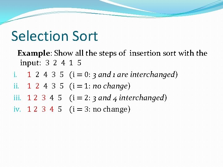
Selection Sort Example: Show all the steps of insertion sort with the input: 3 2 4 1 5 i. 1 2 4 3 5 (i = 0: 3 and 1 are interchanged) ii. 1 2 4 3 5 (i = 1: no change) iii. 1 2 3 4 5 (i = 2: 3 and 4 interchanged) iv. 1 2 3 4 5 (i = 3: no change)

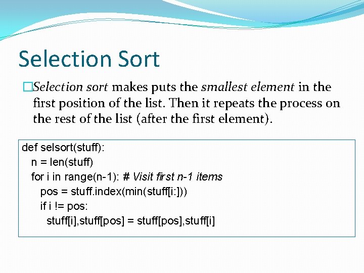
Selection Sort �Selection sort makes puts the smallest element in the first position of the list. Then it repeats the process on the rest of the list (after the first element). def selsort(stuff): n = len(stuff) for i in range(n-1): # Visit first n-1 items pos = stuff. index(min(stuff[i: ])) if i != pos: stuff[i], stuff[pos] = stuff[pos], stuff[i]

Greedy Algorithms �Optimization problems minimize or maximize some parameter over all possible inputs. �Optimization problems can often be solved using a greedy algorithm, which makes the “best” choice at each step. Making the “best choice” at each step does not always produce an optimal solution to the overall problem, but in many instances, it does.

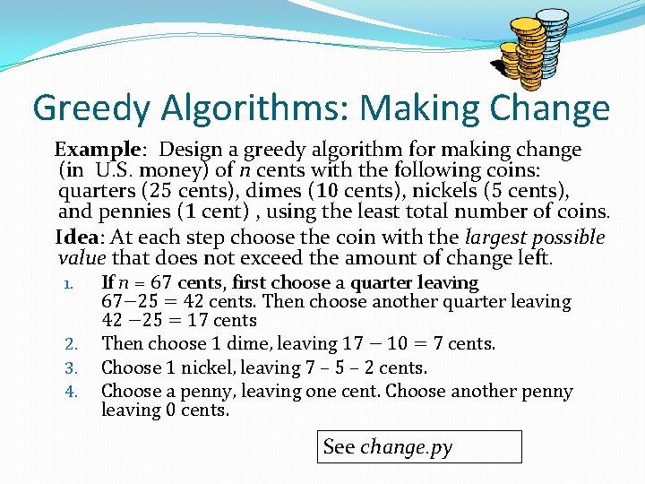
Greedy Algorithms: Making Change Example: Design a greedy algorithm for making change (in U. S. money) of n cents with the following coins: quarters (25 cents), dimes (10 cents), nickels (5 cents), and pennies (1 cent) , using the least total number of coins. Idea: At each step choose the coin with the largest possible value that does not exceed the amount of change left. 1. 2. 3. 4. If n = 67 cents, first choose a quarter leaving 67− 25 = 42 cents. Then choose another quarter leaving 42 − 25 = 17 cents Then choose 1 dime, leaving 17 − 10 = 7 cents. Choose 1 nickel, leaving 7 – 5 – 2 cents. Choose a penny, leaving one cent. Choose another penny leaving 0 cents. See change. py

The Growth of Functions Section 3. 2

Section Summary �Big-O Notation �Big-O Estimates for Important Functions �Big-Omega and Big-Theta Notation

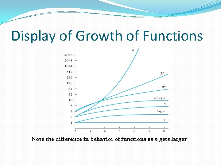
Display of Growth of Functions Note the difference in behavior of functions as n gets larger

The Growth of Functions �In computer science, we want to understand how quickly an algorithm can solve a problem as the size of the input grows. �We can compare the efficiency of two different algorithms for solving the same problem. �We can also determine whether it is practical to use a particular algorithm as the input grows.

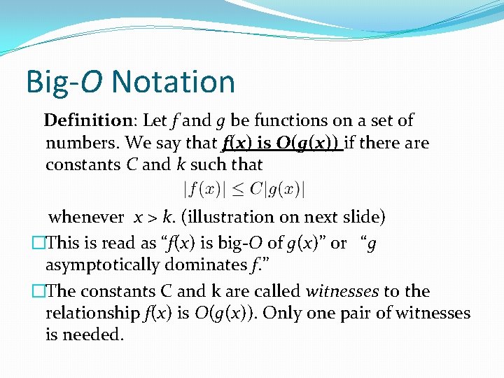
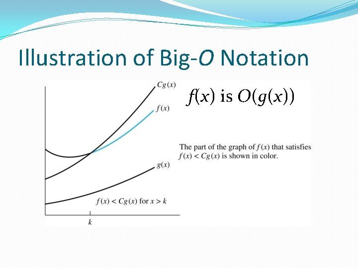
Big-O Notation Definition: Let f and g be functions on a set of numbers. We say that f(x) is O(g(x)) if there are constants C and k such that whenever x > k. (illustration on next slide) �This is read as “f(x) is big-O of g(x)” or “g asymptotically dominates f. ” �The constants C and k are called witnesses to the relationship f(x) is O(g(x)). Only one pair of witnesses is needed.

Illustration of Big-O Notation f(x) is O(g(x))

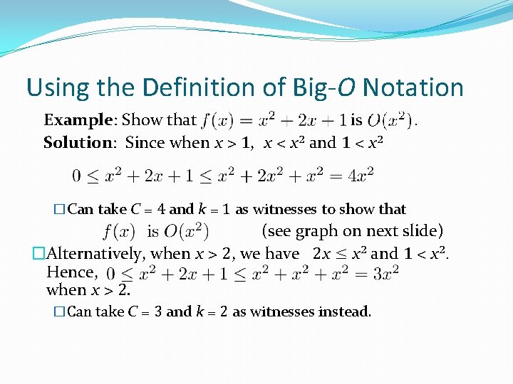
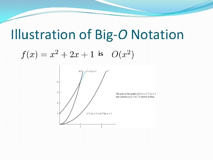
Using the Definition of Big-O Notation Example: Show that is Solution: Since when x > 1, x < x 2 and 1 < x 2 . �Can take C = 4 and k = 1 as witnesses to show that (see graph on next slide) �Alternatively, when x > 2, we have 2 x ≤ x 2 and 1 < x 2. Hence, when x > 2. �Can take C = 3 and k = 2 as witnesses instead.

Illustration of Big-O Notation is

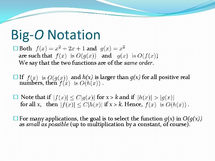
Big-O Notation � Both and are such that and. We say that the two functions are of the same order. � If numbers, then � Note that if for all x, then and h(x) is larger than g(x) for all positive real. for x > k and if if x > k. Hence, . � For many applications, the goal is to select the function g(x) in O(g(x)) as small as possible (up to multiplication by a constant, of course).

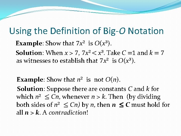
Using the Definition of Big-O Notation Example: Show that 7 x 2 is O(x 3). Solution: When x > 7, 7 x 2 < x 3. Take C =1 and k = 7 as witnesses to establish that 7 x 2 is O(x 3). Example: Show that n 2 is not O(n). Solution: Suppose there are constants C and k for which n 2 ≤ Cn, whenever n > k. Then (by dividing both sides of n 2 ≤ Cn) by n, then n ≤ C must hold for all n > k. A contradiction!

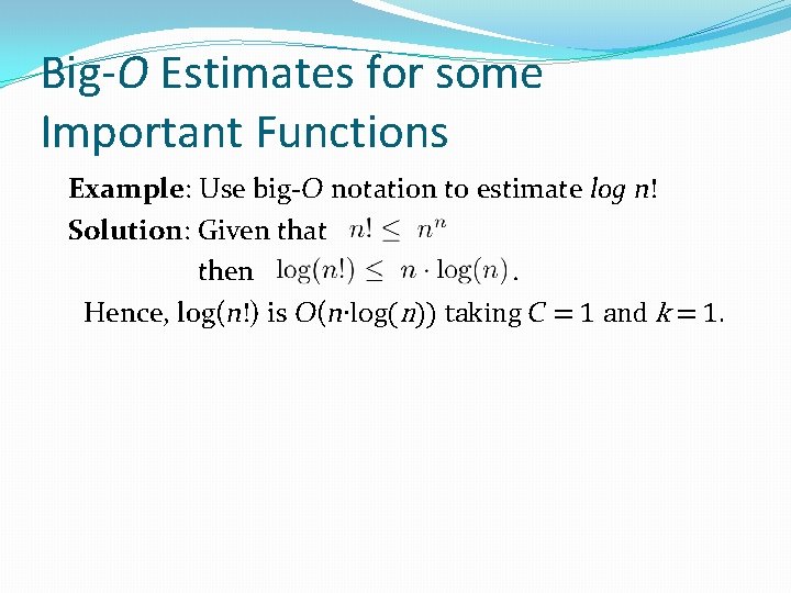
Big-O Estimates for some Important Functions Example: Use big-O notation to estimate log n! Solution: Given that then. Hence, log(n!) is O(n∙log(n)) taking C = 1 and k = 1.

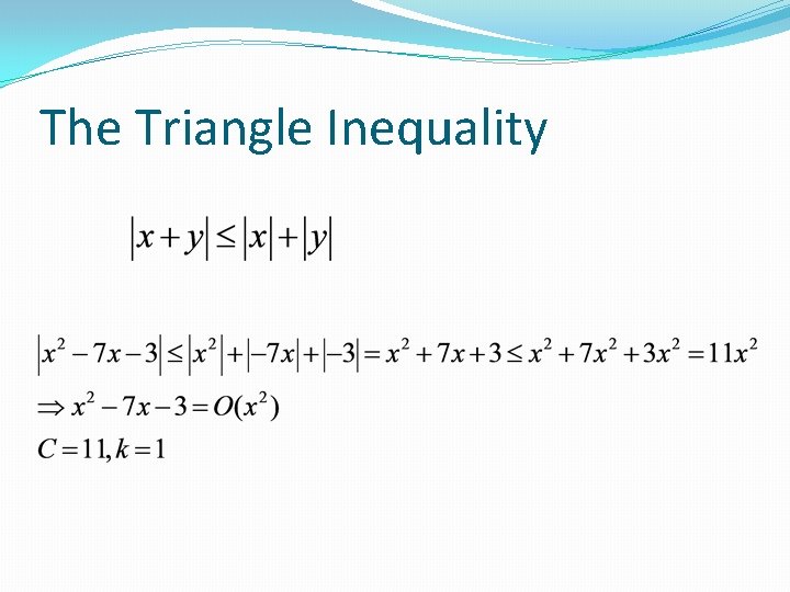
The Triangle Inequality

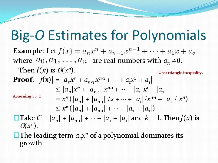
Big-O Estimates for Polynomials Example: Let where are real numbers with an ≠ 0. Then f(x) is O(xn). Uses triangle inequality. Proof: |f(x)| = |anxn + an-1 xn-1 + ∙∙∙ + a 1 x 1 + a 1| ≤ |an|xn + |an-1| xn-1 + ∙∙∙ + |a 1|x 1 + |a 1| Assuming x > 1 = xn (|an| + |an-1| /x + ∙∙∙ + |a 1|/xn-1 + |a 1|/ xn) ≤ xn (|an| + |an-1| + ∙∙∙ + |a 1|) �Take C = |an| + |an-1| + ∙∙∙ + |a 1| and k = 1. Then f(x) is O(xn). �The leading term anxn of a polynomial dominates its growth.

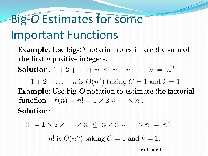
Big-O Estimates for some Important Functions Example: Use big-O notation to estimate the sum of the first n positive integers. Solution: Example: Use big-O notation to estimate the factorial function Solution: Continued →

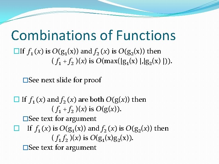
Combinations of Functions �If f 1 (x) is O(g 1(x)) and f 2 (x) is O(g 2(x)) then ( f 1 + f 2 )(x) is O(max(|g 1(x) |, |g 2(x) |)). �See next slide for proof � If f 1 (x) and f 2 (x) are both O(g(x)) then ( f 1 + f 2 )(x) is O(g(x)). �See text for argument � If f 1 (x) is O(g 1(x)) and f 2 (x) is O(g 2(x)) then ( f 1 f 2 )(x) is O(g 1(x)g 2(x)). �See text for argument

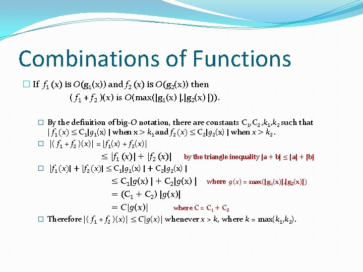
Combinations of Functions � If f 1 (x) is O(g 1(x)) and f 2 (x) is O(g 2(x)) then ( f 1 + f 2 )(x) is O(max(|g 1(x) |, |g 2(x) |)). � By the definition of big-O notation, there are constants C 1, C 2 , k 1, k 2 such that | f 1 (x) ≤ C 1|g 1(x) | when x > k 1 and f 2 (x) ≤ C 2|g 2(x) | when x > k 2. � |( f 1 + f 2 )(x)| = |f 1(x) + f 2(x)| ≤ |f 1 (x)| + |f 2 (x)| by the triangle inequality |a + b| ≤ |a| + |b| � |f 1 (x)| + |f 2 (x)| ≤ C 1|g 1(x) | + C 2|g 2(x) | ≤ C 1|g(x) | + C 2|g(x) | where g(x) = max(|g 1(x)|, |g 2(x)|) = (C 1 + C 2) |g(x)| = C|g(x)| where C = C 1 + C 2 � Therefore |( f 1 + f 2 )(x)| ≤ C|g(x)| whenever x > k, where k = max(k 1, k 2).

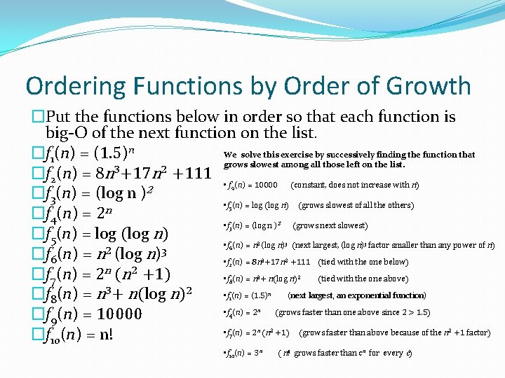
Ordering Functions by Order of Growth �Put the functions below in order so that each function is big-O of the next function on the list. We solve this exercise by successively finding the function that �f 1(n) = (1. 5)n grows slowest among all those left on the list. 3 2 �f 2(n) = 8 n +17 n +111 • f (n) = 10000 (constant, does not increase with n) �f 3(n) = (log n )2 • f (n) = log (log n) (grows slowest of all the others) n �f 4(n) = 2 • f (n) = (log n ) (grows next slowest) �f 5(n) = log (log n) • f (n) = n (log n) (next largest, (log n) factor smaller than any power of n) 2 3 �f 6(n) = n (log n) • f (n) = 8 n +17 n +111 (tied with the one below) n 2 �f 7(n) = 2 (n +1) • f (n) = n + n(log n) (tied with the one above) • f (n) = (1. 5) (next largest, an exponential function) �f 8(n) = n 3+ n(log n)2 • f (n) = 2 (grows faster than one above since 2 > 1. 5) �f 9(n) = 10000 • f (n) = 2 (n +1) (grows faster than above because of the n +1 factor) �f 10(n) = n! 9 5 2 3 6 3 2 8 3 2 7 2 3 2 n 1 4 3 n n • f 10(n) = 3 n 2 2 ( n! grows faster than cn for every c)

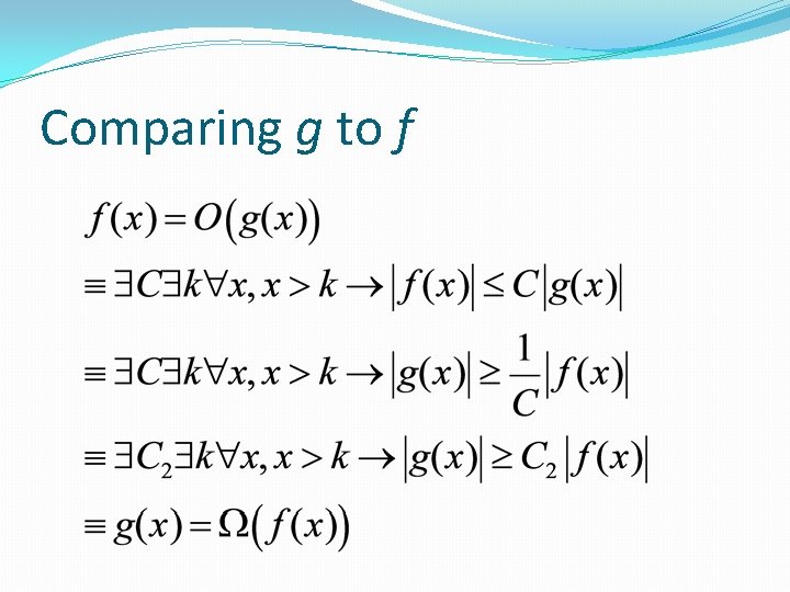
Comparing g to f

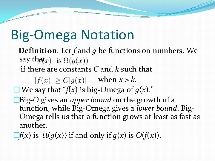
Big-Omega Notation Definition: Let f and g be functions on numbers. We say that if there are constants C and k such that when x > k. � We say that “f(x) is big-Omega of g(x). ” �Big-O gives an upper bound on the growth of a function, while Big-Omega gives a lower bound. Big. Omega tells us that a function grows at least as fast as another. �f(x) is Ω(g(x)) if and only if g(x) is O(f(x)).

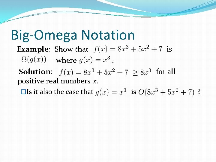
Big-Omega Notation Example: Show that where Solution: positive real numbers x. �Is it also the case that is. for all is ?

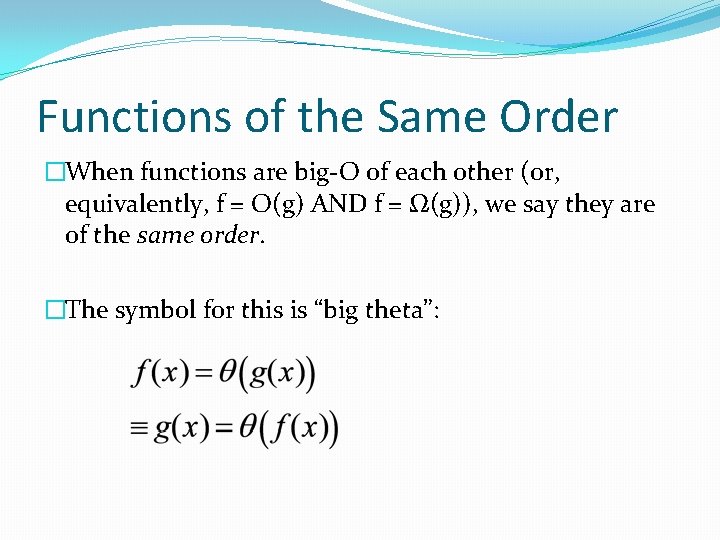
Functions of the Same Order �When functions are big-O of each other (or, equivalently, f = O(g) AND f = Ω(g)), we say they are of the same order. �The symbol for this is “big theta”:

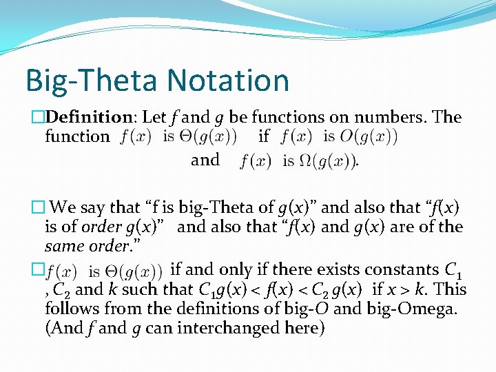
Big-Theta Notation �Definition: Let f and g be functions on numbers. The function if and. � We say that “f is big-Theta of g(x)” and also that “f(x) is of order g(x)” and also that “f(x) and g(x) are of the same order. ” � if and only if there exists constants C 1 , C 2 and k such that C 1 g(x) < f(x) < C 2 g(x) if x > k. This follows from the definitions of big-O and big-Omega. (And f and g can interchanged here)

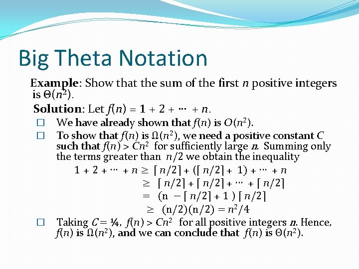
Big Theta Notation Example: Show that the sum of the first n positive integers is Θ(n 2). Solution: Let f(n) = 1 + 2 + ∙∙∙ + n. We have already shown that f(n) is O(n 2). To show that f(n) is Ω(n 2), we need a positive constant C such that f(n) > Cn 2 for sufficiently large n. Summing only the terms greater than n/2 we obtain the inequality 1 + 2 + ∙∙∙ + n ≥ ⌈ n/2⌉ + (⌈ n/2⌉ + 1) + ∙∙∙ + n ≥ ⌈ n/2⌉ + ∙∙∙ + ⌈ n/2⌉ = (n − ⌈ n/2⌉ + 1 ) ⌈ n/2⌉ ≥ (n/2) = n 2/4 � Taking C = ¼, f(n) > Cn 2 for all positive integers n. Hence, f(n) is Ω(n 2), and we can conclude that f(n) is Θ(n 2). � �

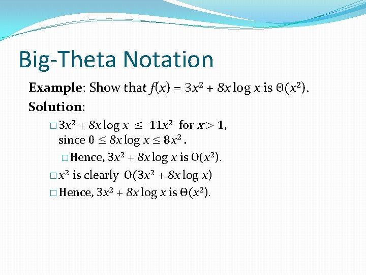
Big-Theta Notation Example: Sh 0 w that f(x) = 3 x 2 + 8 x log x is Θ(x 2). Solution: � 3 x 2 + 8 x log x ≤ 11 x 2 for x > 1, since 0 ≤ 8 x log x ≤ 8 x 2. � Hence, 3 x 2 + 8 x log x is O(x 2). � x 2 is clearly O(3 x 2 + 8 x log x) � Hence, 3 x 2 + 8 x log x is Θ(x 2).

Complexity of Algorithms Section 3. 3

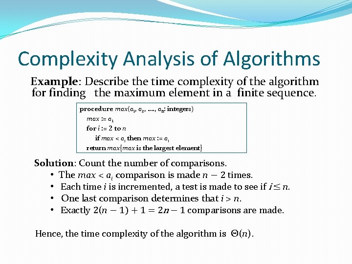
Complexity Analysis of Algorithms Example: Describe the time complexity of the algorithm for finding the maximum element in a finite sequence. procedure max(a 1, a 2, …. , an: integers) max : = a 1 for i : = 2 to n if max < ai then max : = ai return max{max is the largest element} Solution: Count the number of comparisons. • The max < ai comparison is made n − 2 times. • Each time i is incremented, a test is made to see if i ≤ n. • One last comparison determines that i > n. • Exactly 2(n − 1) + 1 = 2 n − 1 comparisons are made. Hence, the time complexity of the algorithm is Θ(n).

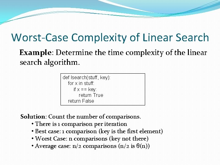
Worst-Case Complexity of Linear Search Example: Determine the time complexity of the linear search algorithm. def lsearch(stuff, key): for x in stuff: if x == key: return True return False Solution: Count the number of comparisons. • There is 1 comparison per iteration • Best case: 1 comparison (key is the first element) • Worst Case: n comparisons (key not there) • Average case: n/2 comparisons (n/2 is θ(n))

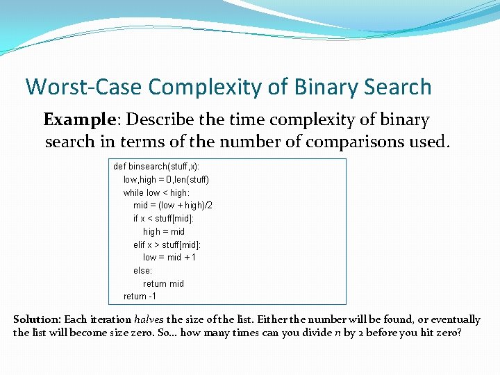
Worst-Case Complexity of Binary Search Example: Describe the time complexity of binary search in terms of the number of comparisons used. def binsearch(stuff, x): low, high = 0, len(stuff) while low < high: mid = (low + high)/2 if x < stuff[mid]: high = mid elif x > stuff[mid]: low = mid + 1 else: return mid return -1 Solution: Each iteration halves the size of the list. Either the number will be found, or eventually the list will become size zero. So… how many times can you divide n by 2 before you hit zero?

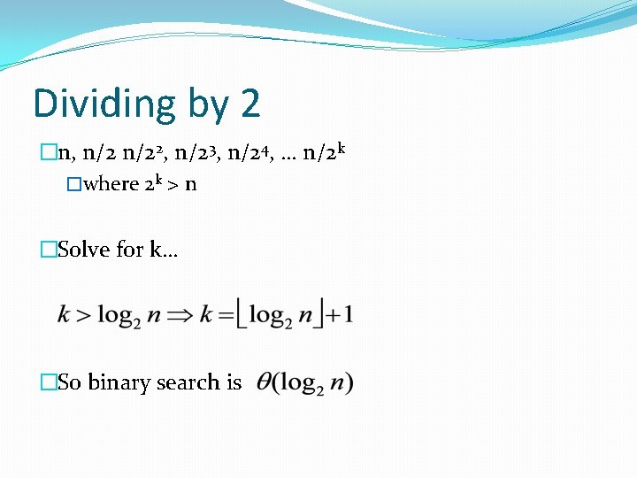
Dividing by 2 �n, n/22, n/23, n/24, … n/2 k �where 2 k > n �Solve for k… �So binary search is

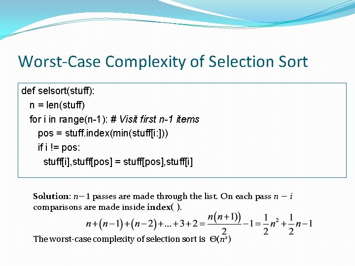
Worst-Case Complexity of Selection Sort def selsort(stuff): n = len(stuff) for i in range(n-1): # Visit first n-1 items pos = stuff. index(min(stuff[i: ])) if i != pos: stuff[i], stuff[pos] = stuff[pos], stuff[i] Solution: n− 1 passes are made through the list. On each pass n − i comparisons are made inside index( ). The worst-case complexity of selection sort is Θ(n 2)

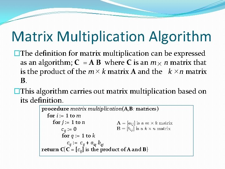
Matrix Multiplication Algorithm �The definition for matrix multiplication can be expressed as an algorithm; C = A B where C is an m n matrix that is the product of the m k matrix A and the k n matrix B. �This algorithm carries out matrix multiplication based on its definition. procedure matrix multiplication(A, B: matrices) for i : = 1 to m for j : = 1 to n cij : = 0 for q : = 1 to k cij : = cij + aiq bqj return C{C = [cij] is the product of A and B}

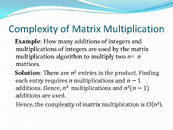
Complexity of Matrix Multiplication Example: How many additions of integers and multiplications of integers are used by the matrix multiplication algorithm to multiply two n n matrices. Solution: There are n 2 entries in the product. Finding each entry requires n multiplications and n − 1 additions. Hence, n 3 multiplications and n 2(n − 1) additions are used. Hence, the complexity of matrix multiplication is O(n 3).

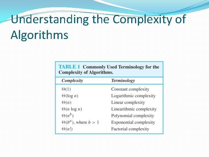
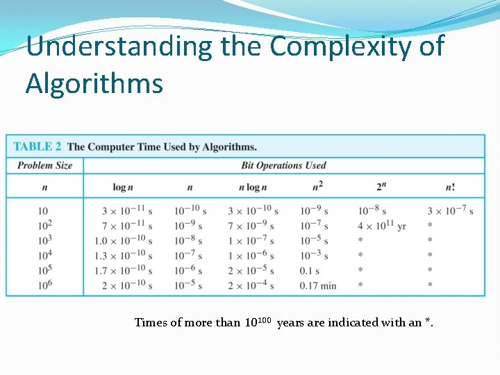
Understanding the Complexity of Algorithms

Understanding the Complexity of Algorithms Times of more than 10100 years are indicated with an *.