ANALYSIS AND DESIGN OF ALGORITHMS UNITII CHAPTER 5
![Insertion Sort As shown in below figure, starting with A[1] and ending with A[n Insertion Sort As shown in below figure, starting with A[1] and ending with A[n](https://slidetodoc.com/presentation_image_h/0f404cbd3a643834ed365b12e068055b/image-14.jpg)
![Insertion Sort Example: Insert Action: i=1, first iteration v a[0] a[1] a[2] a[3] a[4] Insertion Sort Example: Insert Action: i=1, first iteration v a[0] a[1] a[2] a[3] a[4]](https://slidetodoc.com/presentation_image_h/0f404cbd3a643834ed365b12e068055b/image-18.jpg)
![Insertion Sort Example: Insert Action: i=2, second iteration v a[0] a[1] a[2] a[3] a[4] Insertion Sort Example: Insert Action: i=2, second iteration v a[0] a[1] a[2] a[3] a[4]](https://slidetodoc.com/presentation_image_h/0f404cbd3a643834ed365b12e068055b/image-19.jpg)
![Insertion Sort Example: Insert Action: i=3, third iteration v a[0] a[1] a[2] a[3] a[4] Insertion Sort Example: Insert Action: i=3, third iteration v a[0] a[1] a[2] a[3] a[4]](https://slidetodoc.com/presentation_image_h/0f404cbd3a643834ed365b12e068055b/image-20.jpg)
![Insertion Sort Example: Insert Action: i=4, fourth iteration v a[0] a[1] a[2] a[3] a[4] Insertion Sort Example: Insert Action: i=4, fourth iteration v a[0] a[1] a[2] a[3] a[4]](https://slidetodoc.com/presentation_image_h/0f404cbd3a643834ed365b12e068055b/image-21.jpg)
![Insertion Sort Analysis: In the Best case, the comparison A[j] > v is executed Insertion Sort Analysis: In the Best case, the comparison A[j] > v is executed](https://slidetodoc.com/presentation_image_h/0f404cbd3a643834ed365b12e068055b/image-26.jpg)
- Slides: 101

ANALYSIS AND DESIGN OF ALGORITHMS UNIT-II CHAPTER 5: DECREASE-AND-CONQUER

OUTLINE : Ø Decrease-and-Conquer • • • Insertion Sort Depth-First Search Breadth-First Search Topological Sorting Algorithms for Generating Combinatorial Objects § § Generating Permutations Generating Subsets

Decrease-and-Conquer Ø The decrease-and-Conquer technique is based on exploiting the relationship between a solution to a given instance of a problem and a solution to a smaller instance of the same problem. Ø Once such a relationship is established, it can be exploited either top down (recursively) or bottom up (without a recursion).

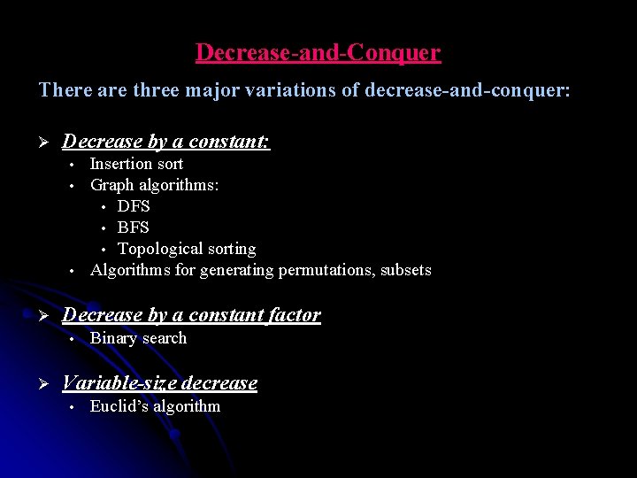
Decrease-and-Conquer There are three major variations of decrease-and-conquer: Ø Decrease by a constant: • • • Ø Decrease by a constant factor • Ø Insertion sort Graph algorithms: • DFS • BFS • Topological sorting Algorithms for generating permutations, subsets Binary search Variable-size decrease • Euclid’s algorithm

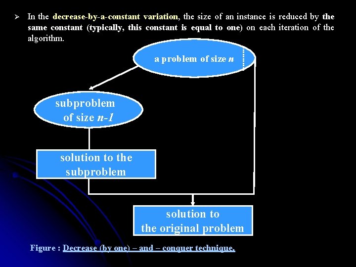
Ø In the decrease-by-a-constant variation, the size of an instance is reduced by the same constant (typically, this constant is equal to one) on each iteration of the algorithm. a problem of size n subproblem of size n-1 solution to the subproblem solution to the original problem Figure : Decrease (by one) – and – conquer technique.

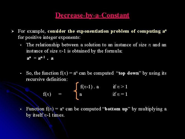
Decrease-by-a-Constant Ø For example, consider the exponentiation problem of computing an for positive integer exponents: • The relationship between a solution to an instance of size n and an instance of size n-1 is obtained by the formula: an = an-1. a So, the function f(n) = an can be computed “top down” by using its recursive definition: f(n-1). a if n > 1 f(n) = a if n = 1 • • Function f(n) = an can be computed “bottom up” by multiplying a by itself n-1 times.

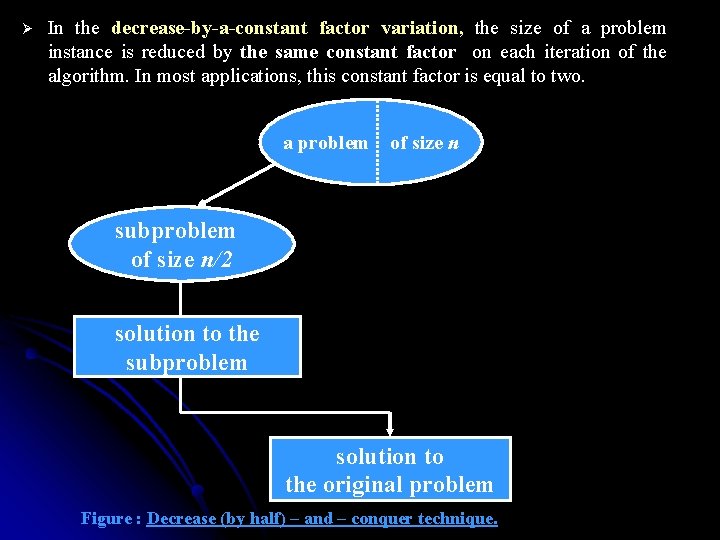
Ø In the decrease-by-a-constant factor variation, the size of a problem instance is reduced by the same constant factor on each iteration of the algorithm. In most applications, this constant factor is equal to two. a problem of size n subproblem of size n/2 solution to the subproblem solution to the original problem Figure : Decrease (by half) – and – conquer technique.

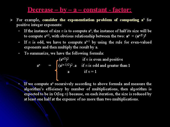
Decrease – by – a – constant - factor: For example, consider the exponentiation problem of computing an for positive integer exponents: • If the instance of size n is to compute an, the instance of half its size will be to compute an/2, with obvious relationship between the two: an = (an/2 )2 • If n is odd, we have to compute an-1 by using the rule for even-valued exponents and then multiply the result by a. • To summarize, we have the following formula: (an/2)2 if n is even and positive an = (a(n-1)/2)2. a if n is odd and greater than 1 a if n = 1 Ø • If we compute an recursively according to above formula and measure the algorithm’s efficiency by number of multiplications, then algorithm is expected to be in O(log n) because, on each iteration, the size is reduced by at least one half at the expense of no more than two multiplications.

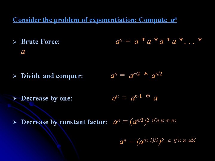
Consider the problem of exponentiation: Compute an Ø Brute Force: an = a * a *. . . * a Ø Divide and conquer: an = an/2 * an/2 Ø Decrease by one: an = an-1 * a Ø Decrease by constant factor: an = (an/2)2 if n is even an = (a(n-1)/2)2. a if n is odd

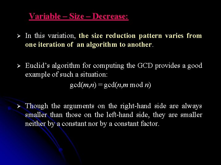
Variable – Size – Decrease: Ø In this variation, the size reduction pattern varies from one iteration of an algorithm to another. Ø Euclid’s algorithm for computing the GCD provides a good example of such a situation: gcd(m, n) = gcd(n, m mod n) Though the arguments on the right-hand side are always smaller than those on the left-hand side, they are smaller neither by a constant nor by a constant factor. Ø

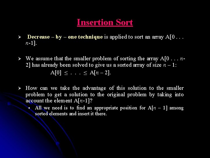
Insertion Sort Ø Decrease – by – one technique is applied to sort an array A[0. . . n-1]. Ø We assume that the smaller problem of sorting the array A[0. . . n 2] has already been solved to give us a sorted array of size n – 1: A[0] ≤ . . . ≤ A[n – 2]. Ø How can we take the advantage of this solution to the smaller problem to get a solution to the original problem by taking into account the element A[n-1]? § All we need is to find an appropriate position for A[n – 1] among sorted elements and insert it there.

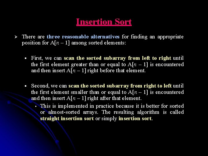
Insertion Sort Ø There are three reasonable alternatives for finding an appropriate position for A[n – 1] among sorted elements: § First, we can scan the sorted subarray from left to right until the first element greater than or equal to A[n – 1] is encountered and then insert A[n – 1] right before that element. § Second, we can scan the sorted subarray from right to left until the first element smaller than or equal to A[n – 1] is encountered and then insert A[n – 1] right after that element. • This is implemented in practice because it is better for sorted or almost-sorted arrays. The resulting algorithm is called straight insertion sort or simply insertion sort.

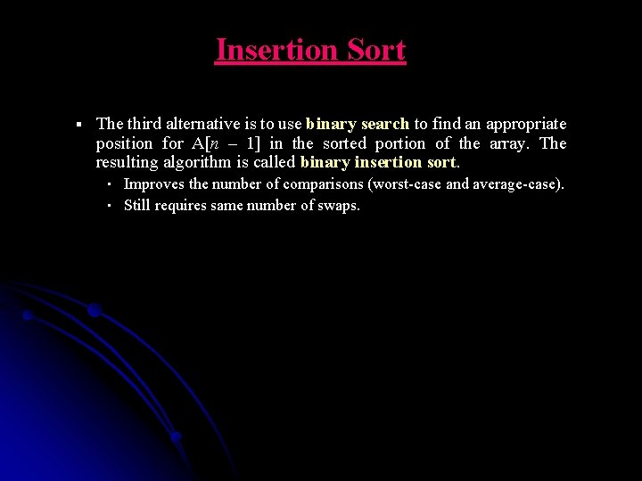
Insertion Sort § The third alternative is to use binary search to find an appropriate position for A[n – 1] in the sorted portion of the array. The resulting algorithm is called binary insertion sort. • • Improves the number of comparisons (worst-case and average-case). Still requires same number of swaps.
![Insertion Sort As shown in below figure starting with A1 and ending with An Insertion Sort As shown in below figure, starting with A[1] and ending with A[n](https://slidetodoc.com/presentation_image_h/0f404cbd3a643834ed365b12e068055b/image-14.jpg)
Insertion Sort As shown in below figure, starting with A[1] and ending with A[n – 1], A[i] is inserted in its appropriate place among the first i elements of the array that have been already sorted (but, unlike selection sort, are generally not in their final positions). A[0] ≤ . . . ≤ A[j] < A[j + 1] ≤ . . . ≤ A[i – 1] | A[i]. . . A[n – 1] Smaller than or equal to A[i] greater than A[i]

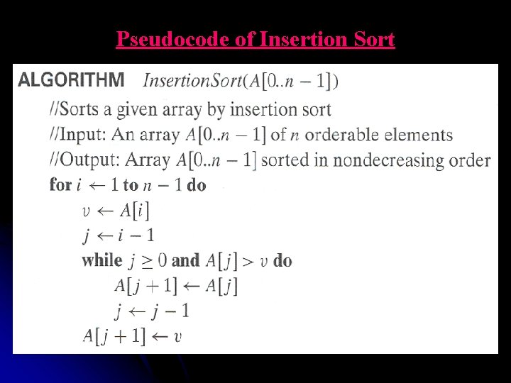
Pseudocode of Insertion Sort

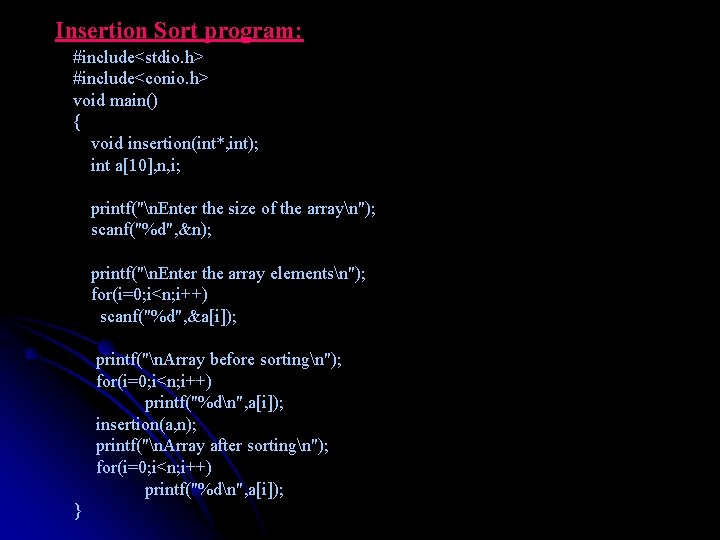
Insertion Sort program: #include<stdio. h> #include<conio. h> void main() { void insertion(int*, int); int a[10], n, i; printf("n. Enter the size of the arrayn"); scanf("%d", &n); printf("n. Enter the array elementsn"); for(i=0; i<n; i++) scanf("%d", &a[i]); printf("n. Array before sortingn"); for(i=0; i<n; i++) printf("%dn", a[i]); insertion(a, n); printf("n. Array after sortingn"); for(i=0; i<n; i++) printf("%dn", a[i]); }

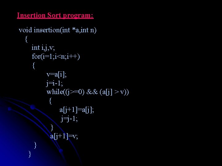
Insertion Sort program: void insertion(int *a, int n) { int i, j, v; for(i=1; i<n; i++) { v=a[i]; j=i-1; while((j>=0) && (a[j] > v)) { a[j+1]=a[j]; j=j-1; } a[j+1]=v; } }
![Insertion Sort Example Insert Action i1 first iteration v a0 a1 a2 a3 a4 Insertion Sort Example: Insert Action: i=1, first iteration v a[0] a[1] a[2] a[3] a[4]](https://slidetodoc.com/presentation_image_h/0f404cbd3a643834ed365b12e068055b/image-18.jpg)
Insertion Sort Example: Insert Action: i=1, first iteration v a[0] a[1] a[2] a[3] a[4] 8 20 8 5 10 7 8 20 20 5 10 7 8 8 20 5 10 7
![Insertion Sort Example Insert Action i2 second iteration v a0 a1 a2 a3 a4 Insertion Sort Example: Insert Action: i=2, second iteration v a[0] a[1] a[2] a[3] a[4]](https://slidetodoc.com/presentation_image_h/0f404cbd3a643834ed365b12e068055b/image-19.jpg)
Insertion Sort Example: Insert Action: i=2, second iteration v a[0] a[1] a[2] a[3] a[4] 5 8 20 5 10 7 5 8 20 20 10 7 5 8 8 20 10 7 5 5 8 20 10 7
![Insertion Sort Example Insert Action i3 third iteration v a0 a1 a2 a3 a4 Insertion Sort Example: Insert Action: i=3, third iteration v a[0] a[1] a[2] a[3] a[4]](https://slidetodoc.com/presentation_image_h/0f404cbd3a643834ed365b12e068055b/image-20.jpg)
Insertion Sort Example: Insert Action: i=3, third iteration v a[0] a[1] a[2] a[3] a[4] 10 5 8 20 10 7 10 5 8 20 20 7 10 5 8 10 20 7
![Insertion Sort Example Insert Action i4 fourth iteration v a0 a1 a2 a3 a4 Insertion Sort Example: Insert Action: i=4, fourth iteration v a[0] a[1] a[2] a[3] a[4]](https://slidetodoc.com/presentation_image_h/0f404cbd3a643834ed365b12e068055b/image-21.jpg)
Insertion Sort Example: Insert Action: i=4, fourth iteration v a[0] a[1] a[2] a[3] a[4] 7 5 8 10 20 7 7 5 8 10 20 20 7 5 8 10 10 20 7 5 8 8 10 20 7 5 7 8 10 20 Sorted ARRAY

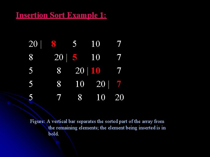
Insertion Sort Example 1: 20 | 8 5 10 7 8 20 | 5 10 7 5 8 20 | 10 7 5 8 10 20 | 7 5 7 8 10 20 Figure: A vertical bar separates the sorted part of the array from the remaining elements; the element being inserted is in bold.

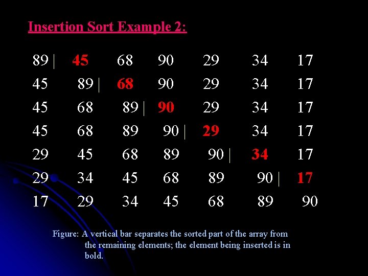
Insertion Sort Example 2: 89 | 45 68 90 29 34 17 45 89 | 68 90 29 34 17 45 68 89 | 90 29 34 17 45 68 89 90 | 29 34 17 29 45 68 89 90 | 34 17 29 34 45 68 89 90 | 17 17 29 34 45 68 89 90 Figure: A vertical bar separates the sorted part of the array from the remaining elements; the element being inserted is in bold.

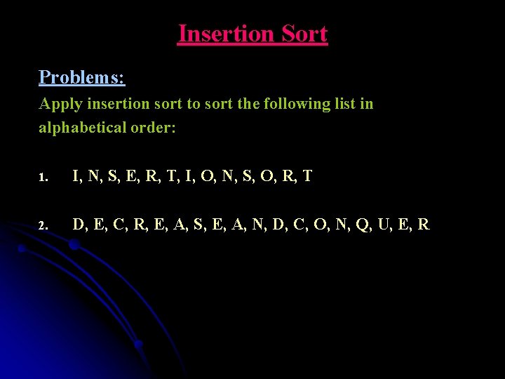
Insertion Sort Problems: Apply insertion sort to sort the following list in alphabetical order: 1. I, N, S, E, R, T, I, O, N, S, O, R, T 2. D, E, C, R, E, A, S, E, A, N, D, C, O, N, Q, U, E, R

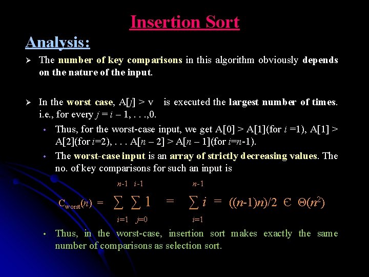
Insertion Sort Analysis: Ø The number of key comparisons in this algorithm obviously depends on the nature of the input. In the worst case, A[j] > v is executed the largest number of times. i. e. , for every j = i – 1, . . . , 0. • Thus, for the worst-case input, we get A[0] > A[1](for i =1), A[1] > A[2](for i=2), . . . A[n – 2] > A[n – 1](for i=n-1). • The worst-case input is an array of strictly decreasing values. The no. of key comparisons for such an input is n-1 i-1 n-1 Ø Cworst(n) = ∑ ∑ 1 = ∑ i = ((n-1)n)/2 Є Θ(n 2) i=1 j=0 i=1 • Thus, in the worst-case, insertion sort makes exactly the same number of comparisons as selection sort.
![Insertion Sort Analysis In the Best case the comparison Aj v is executed Insertion Sort Analysis: In the Best case, the comparison A[j] > v is executed](https://slidetodoc.com/presentation_image_h/0f404cbd3a643834ed365b12e068055b/image-26.jpg)
Insertion Sort Analysis: In the Best case, the comparison A[j] > v is executed only once on every iteration of outer loop. • It happens if and only if A[i – 1] ≤ A[i] for every i = 1, . . . n – 1, i. e. , if the input array is already sorted in ascending order. n-1 Cbest(n) = ∑ 1 = n - 1 Є Θ(n) i=1 Ø

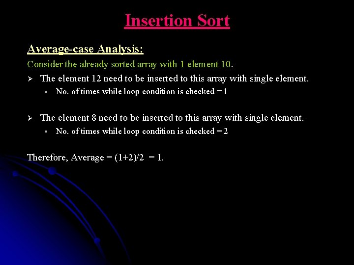
Insertion Sort Average-case Analysis: Consider the already sorted array with 1 element 10. Ø The element 12 need to be inserted to this array with single element. § Ø No. of times while loop condition is checked = 1 The element 8 need to be inserted to this array with single element. § No. of times while loop condition is checked = 2 Therefore, Average = (1+2)/2 = 1.

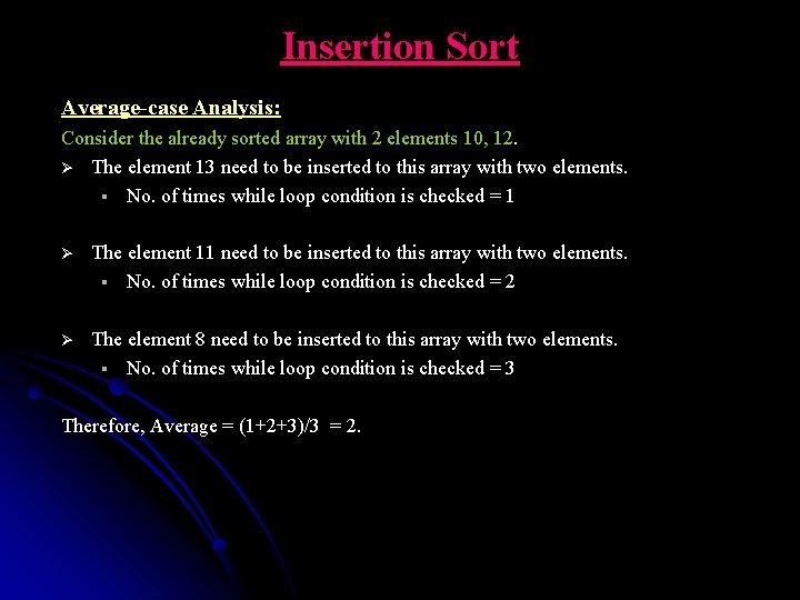
Insertion Sort Average-case Analysis: Consider the already sorted array with 2 elements 10, 12. Ø The element 13 need to be inserted to this array with two elements. § No. of times while loop condition is checked = 1 Ø The element 11 need to be inserted to this array with two elements. § No. of times while loop condition is checked = 2 Ø The element 8 need to be inserted to this array with two elements. § No. of times while loop condition is checked = 3 Therefore, Average = (1+2+3)/3 = 2.

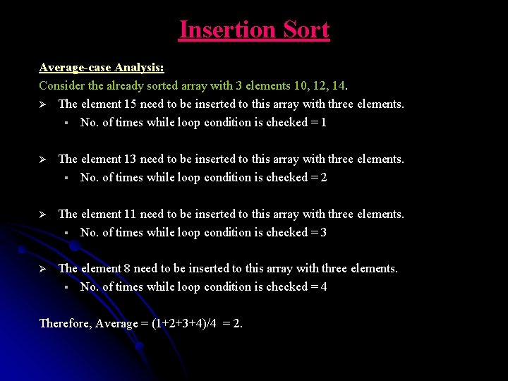
Insertion Sort Average-case Analysis: Consider the already sorted array with 3 elements 10, 12, 14. Ø The element 15 need to be inserted to this array with three elements. § No. of times while loop condition is checked = 1 Ø The element 13 need to be inserted to this array with three elements. § No. of times while loop condition is checked = 2 Ø The element 11 need to be inserted to this array with three elements. § No. of times while loop condition is checked = 3 Ø The element 8 need to be inserted to this array with three elements. § No. of times while loop condition is checked = 4 Therefore, Average = (1+2+3+4)/4 = 2.

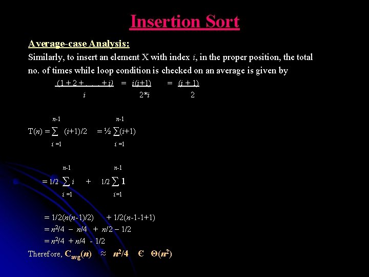
Insertion Sort Average-case Analysis: Similarly, to insert an element X with index i, in the proper position, the total no. of times while loop condition is checked on an average is given by (1 + 2 +. . . + i) = i(i+1) = (i + 1) i 2*i 2 n-1 n-1 T(n) = ∑ (i+1)/2 = ½ ∑(i+1) i =1 n-1 = 1/2 ∑ i + 1/2 ∑ 1 i =1 i=1 = 1/2(n(n-1)/2) + 1/2(n-1 -1+1) = n 2/4 – n/4 + n/2 – 1/2 = n 2/4 + n/4 - 1/2 Therefore, Cavg(n) ≈ n 2/4 Є Θ(n 2)

Graph Traversal Ø Many graph algorithms require processing vertices or edges of a graph in a systematic fashion. Ø There are two principal Graph traversal algorithms: v Depth-first search (DFS) v Breadth-first search (BFS)

Graph Traversal Ø Depth-First Search (DFS) and Breadth-First Search (BFS): • Two elementary traversal algorithms that provide an efficient way to “visit” each vertex and edge exactly once. • Both work on directed or undirected graphs. • Many advanced graph algorithms are based on the concepts of DFS or BFS. • The difference between the two algorithms is in the order in which each “visit” vertices.

Depth-First Search Ø DFS starts visiting vertices of a graph at an arbitrary vertex by marking it as having been visited. Ø On each iteration, the algorithm proceeds to an unvisited vertex that is adjacent to the last visited vertex. Ø This process continues until a dead end – a vertex with no adjacent unvisited vertices – is encountered. Ø At a dead end, the algorithm backs up one edge to the vertex it came from and tries to continue visiting unvisited vertices from there. Ø The algorithm eventually halts after backing up to the starting vertex, with the latter being a dead end.

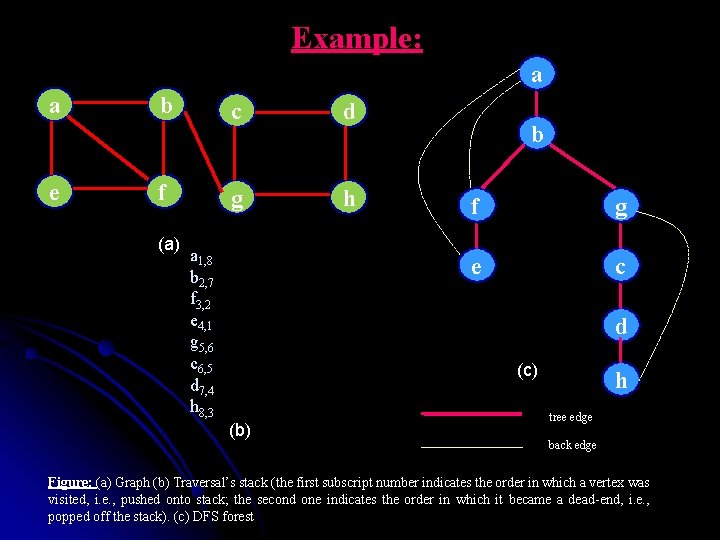
Depth-First Search Ø Ø Ø By this time, all the vertices in the same connected component have been visited. If unvisited vertices still remain, the depth-first search must be restarted at any one of them. It is convenient to use a stack to trace the operation of DFS. We push a vertex onto the stack when the vertex is reached for first time, and we pop a vertex off the stack when it becomes a dead end.

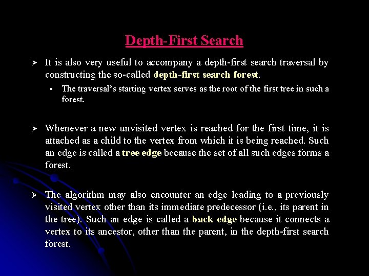
Depth-First Search Ø It is also very useful to accompany a depth-first search traversal by constructing the so-called depth-first search forest. § The traversal’s starting vertex serves as the root of the first tree in such a forest. Ø Whenever a new unvisited vertex is reached for the first time, it is attached as a child to the vertex from which it is being reached. Such an edge is called a tree edge because the set of all such edges forms a forest. Ø The algorithm may also encounter an edge leading to a previously visited vertex other than its immediate predecessor (i. e. , its parent in the tree). Such an edge is called a back edge because it connects a vertex to its ancestor, other than the parent, in the depth-first search forest.

Example: a a e b f (a) c d g h a 1, 8 b 2, 7 f 3, 2 e 4, 1 g 5, 6 c 6, 5 d 7, 4 h 8, 3 b f g e c d (c) (b) h tree edge back edge Figure: (a) Graph (b) Traversal’s stack (the first subscript number indicates the order in which a vertex was visited, i. e. , pushed onto stack; the second one indicates the order in which it became a dead-end, i. e. , popped off the stack). (c) DFS forest

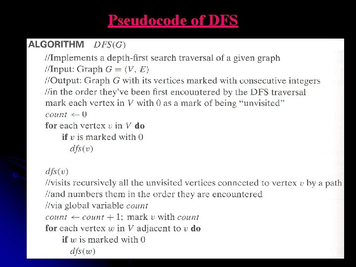
Pseudocode of DFS 37

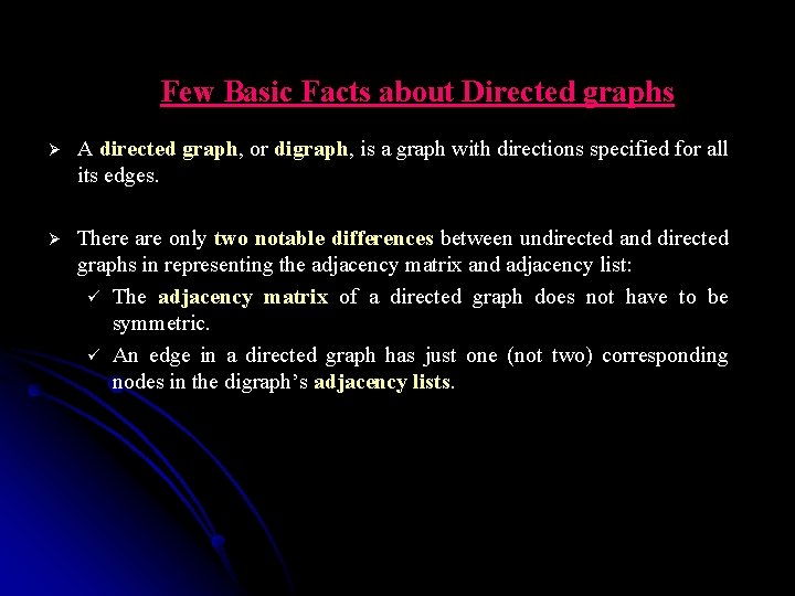
Few Basic Facts about Directed graphs Ø A directed graph, or digraph, is a graph with directions specified for all its edges. Ø There are only two notable differences between undirected and directed graphs in representing the adjacency matrix and adjacency list: ü The adjacency matrix of a directed graph does not have to be symmetric. ü An edge in a directed graph has just one (not two) corresponding nodes in the digraph’s adjacency lists.

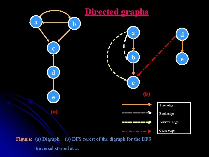
Directed graphs a b a d b e c d c e (b) Tree edge (a) Back edge Forward edge Cross edge Figure: (a) Digraph. (b) DFS forest of the digraph for the DFS traversal started at a.

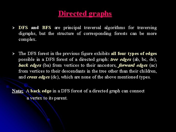
Directed graphs Ø DFS and BFS are principal traversal algorithms for traversing digraphs, but the structure of corresponding forests can be more complex. Ø The DFS forest in the previous figure exhibits all four types of edges possible in a DFS forest of a directed graph: tree edges (ab, bc, de), back edges (ba) from vertices to their ancestors, forward edges (ac) from vertices to their descendants in the tree other than their children, and cross edges (dc), which are none of the above mentioned types. Note: A back edge in a DFS forest of a directed graph can connect a vertex to its parent.

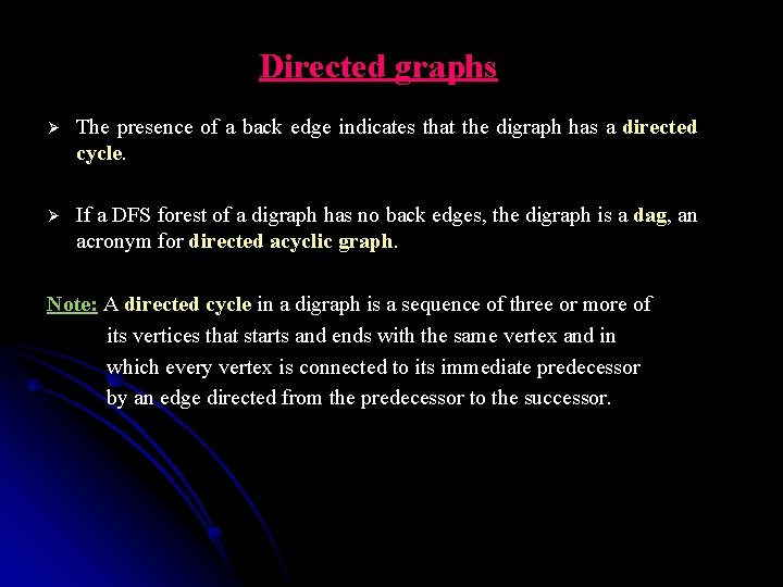
Directed graphs Ø The presence of a back edge indicates that the digraph has a directed cycle. Ø If a DFS forest of a digraph has no back edges, the digraph is a dag, an acronym for directed acyclic graph. Note: A directed cycle in a digraph is a sequence of three or more of its vertices that starts and ends with the same vertex and in which every vertex is connected to its immediate predecessor by an edge directed from the predecessor to the successor.

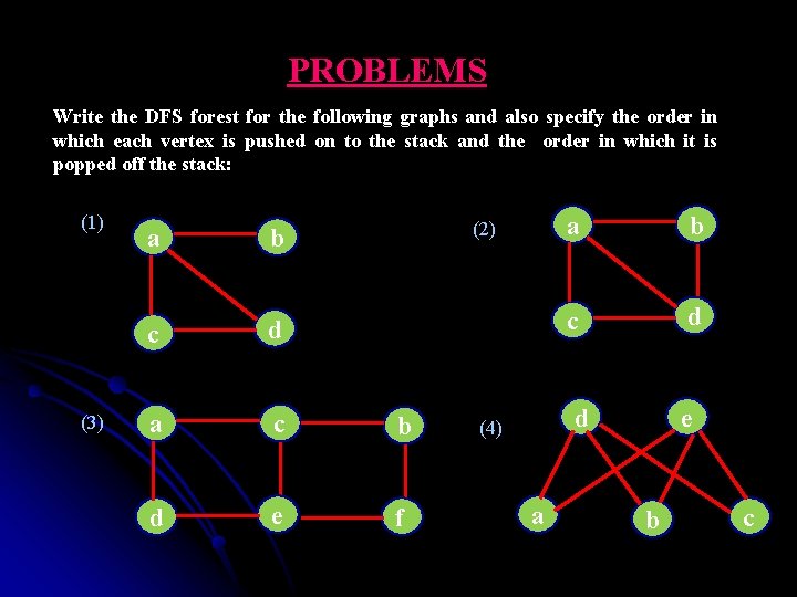
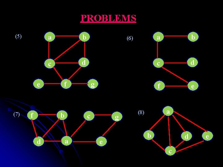
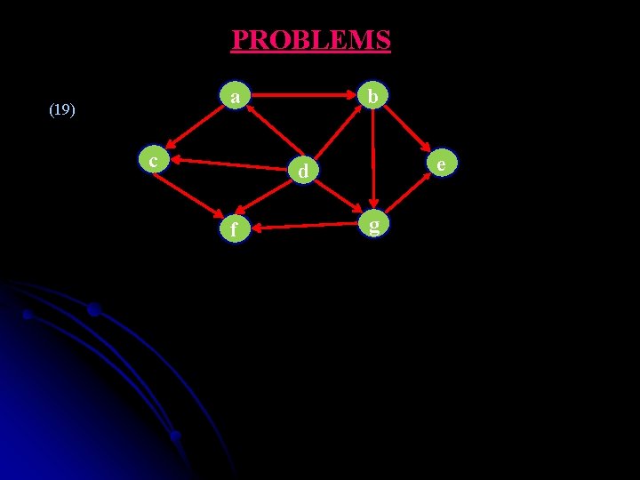
PROBLEMS Write the DFS forest for the following graphs and also specify the order in which each vertex is pushed on to the stack and the order in which it is popped off the stack: (1) (3) (2) a b c d a c b d e f a b c d d (4) a e b c

PROBLEMS (5) e (7) f a b c d f b d (6) g c a g e a b c d f e a (8) b d c e

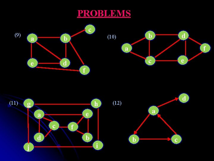
PROBLEMS c (9) a b (10) b d f a (11) f g h d j d (12) a e a c e c d e f b i b c

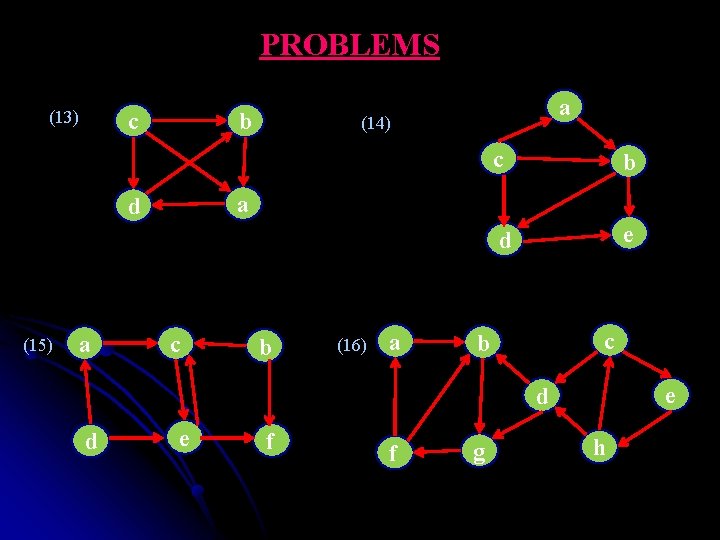
PROBLEMS (13) c b a (14) c b d e a d (15) a c b (16) a c b e d d e f f g h

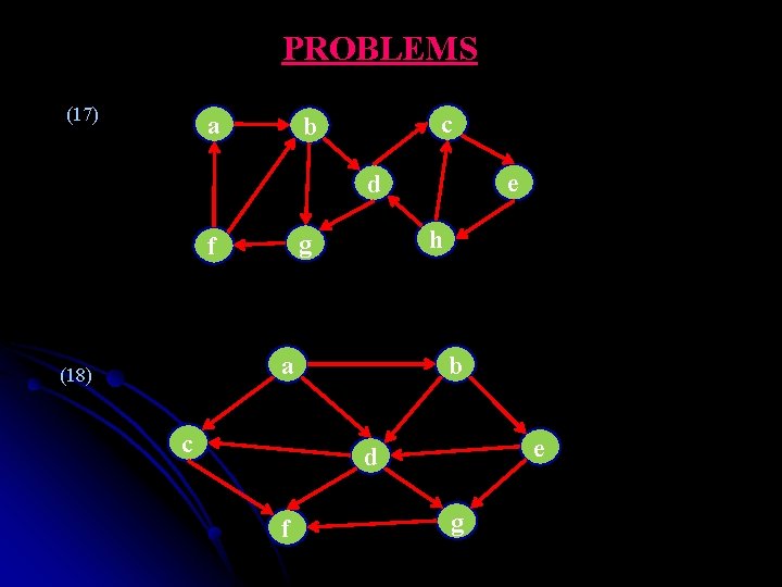
PROBLEMS (17) a c b e d h g f b a (18) c e d f g

PROBLEMS b a (19) c e d f g

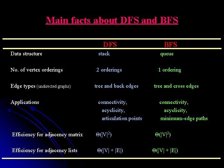
How efficient is Depth-First Search ? Ø DFS algorithm is quite efficient since it takes just the time proportional to the size of the data structure used for representing the graph in question. Ø Thus, for the adjacency matrix representation, the traversal’s time is in Θ(|V|2), and for the adjacency list representation, it is in Θ(|V| + |E|) where |V| and |E| are the number of the graph’s vertices and edges, respectively.

Depth-First Search Ø We can look at the DFS forest as the given graph with its edges classified by the DFS traversal into two disjoint classes: tree edges and back edges. - tree edges are edges used by the DFS traversal to reach previously unvisited vertices. - back edges connect vertices to previously visited vertices other than their immediate predecessors in the traversal. Ø DFS yields two distinct orderings of vertices: - order in which the vertices are reached for the first time (pushed onto stack). - order in which the vertices become dead-ends (popped off stack). These orders are qualitatively different , and various applications can take advantage of either of them.

Applications of DFS Checking connectivity: Since DFS halts after visiting all the vertices connected by a path to the starting vertex, checking a graph’s connectivity can be done as follows: Start a DFS traversal at an arbitrary vertex and check, after the algorithm halts, whether all the graph’s vertices will have been visited. If they have, the graph is connected; otherwise, it is not connected. Ø Ø Identifying connected components of a graph. Ø Checking acyclicity: If the DFS forest does not have back edges, then it is clearly acyclic.

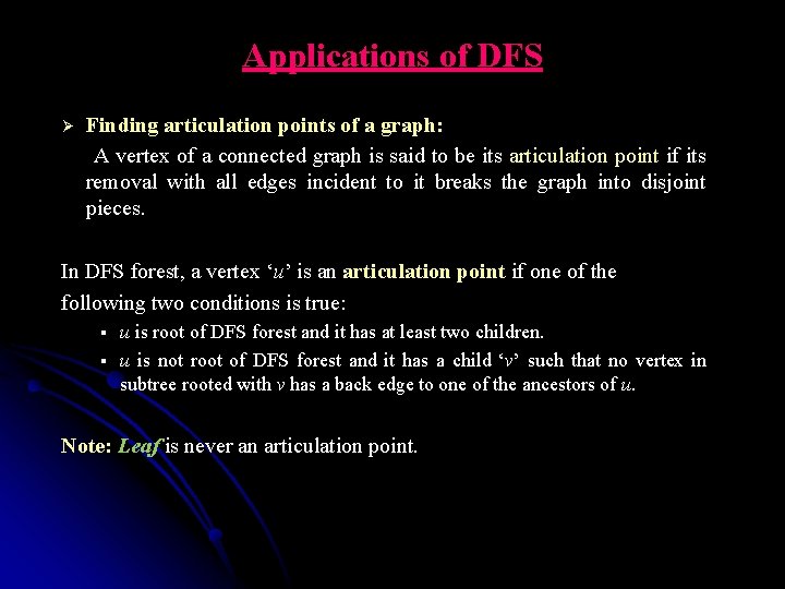
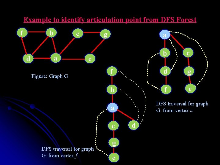
Applications of DFS Finding articulation points of a graph: A vertex of a connected graph is said to be its articulation point if its removal with all edges incident to it breaks the graph into disjoint pieces. Ø In DFS forest, a vertex ‘u’ is an articulation point if one of the following two conditions is true: § § u is root of DFS forest and it has at least two children. u is not root of DFS forest and it has a child ‘v’ such that no vertex in subtree rooted with v has a back edge to one of the ancestors of u. Note: Leaf is never an articulation point.

Example to identify articulation point from DFS Forest f b d c a g a b c f d g b f e e Figure: Graph G DFS traversal for graph G from vertex a a c DFS traversal for graph G from vertex f g e d

Breadth-first search (BFS) Ø It proceeds in a concentric manner by visiting first all the vertices that are adjacent to a starting vertex, then all unvisited vertices two edges apart from it, and so on, until all the vertices in the same connected component as the starting vertex are visited. Ø If unvisited vertices still remain, the algorithm has to be restarted at an arbitrary vertex of another connected component of the graph.

Breadth-first search (BFS) Ø Instead of a stack, BFS uses a queue. The queue is initialized with the traversal’s starting vertex, which is marked as visited. Ø On each iteration, the algorithm identifies all unvisited vertices that are adjacent to the front vertex, marks them as visited, and adds them to the queue; after that, the front vertex is removed from the queue. Ø Similar to level-by-level tree traversal. Ø It is useful to accompany a BFS traversal by constructing the breadth-first search forest. The traversal’s starting vertex serves as the root of the first tree in such a forest.

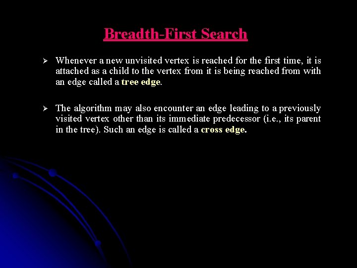
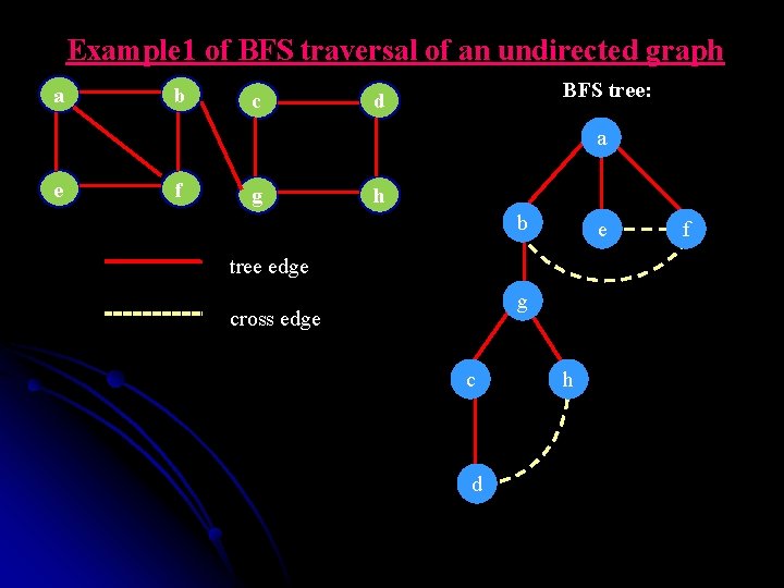
Breadth-First Search Ø Whenever a new unvisited vertex is reached for the first time, it is attached as a child to the vertex from it is being reached from with an edge called a tree edge. Ø The algorithm may also encounter an edge leading to a previously visited vertex other than its immediate predecessor (i. e. , its parent in the tree). Such an edge is called a cross edge.

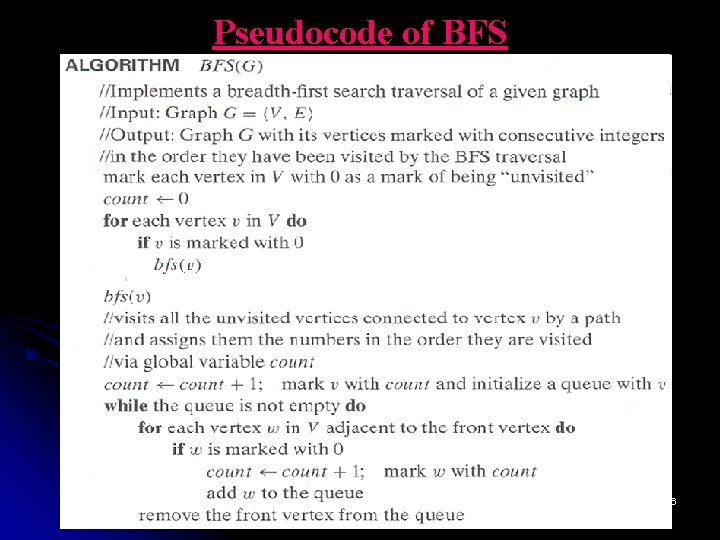
Pseudocode of BFS 56

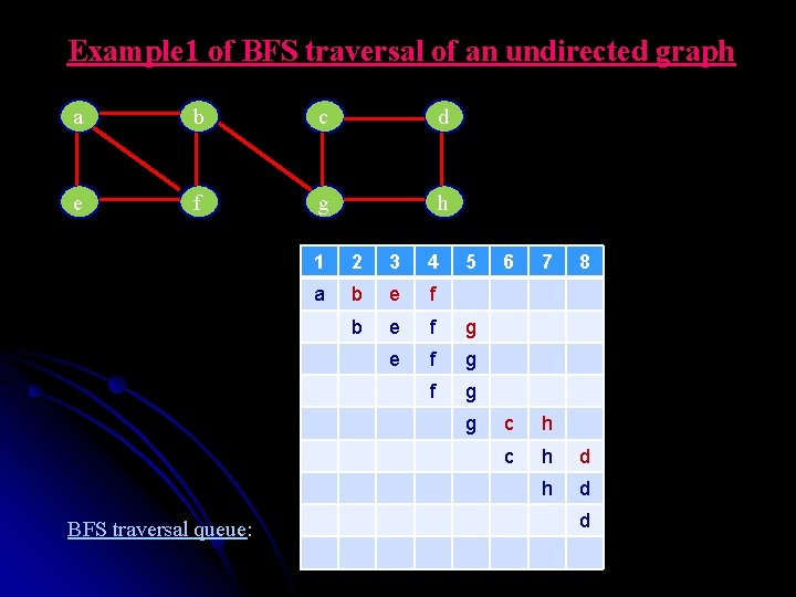
Example 1 of BFS traversal of an undirected graph a b c d e f g h 1 2 3 4 5 a b e f g g BFS traversal queue: 6 7 8 c h d h d d

Example 1 of BFS traversal of an undirected graph a b c BFS tree: d a e f g h b e tree edge g cross edge c d h f

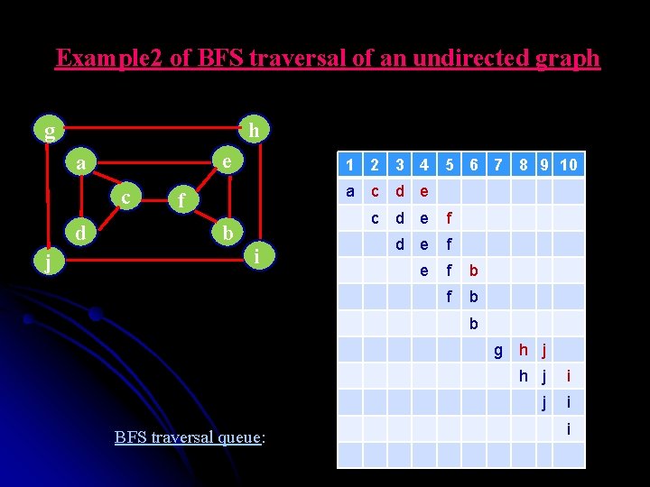
Example 2 of BFS traversal of an undirected graph g h e a c d j 1 2 3 4 5 6 7 8 9 10 a c d e f b i c d e f e f b b g h j BFS traversal queue: h j i i

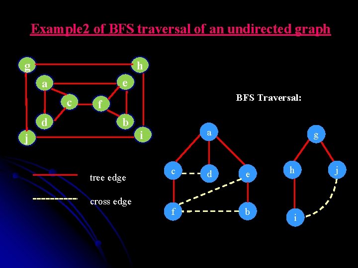
Example 2 of BFS traversal of an undirected graph g h e a c d BFS Traversal: f b j tree edge cross edge a i c f d g e b h i j

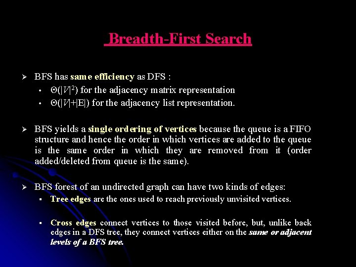
Breadth-First Search Ø BFS has same efficiency as DFS : • Θ(|V|2) for the adjacency matrix representation • Θ(|V|+|E|) for the adjacency list representation. Ø BFS yields a single ordering of vertices because the queue is a FIFO structure and hence the order in which vertices are added to the queue is the same order in which they are removed from it (order added/deleted from queue is the same). Ø BFS forest of an undirected graph can have two kinds of edges: § Tree edges are the ones used to reach previously unvisited vertices. § Cross edges connect vertices to those visited before, but, unlike back edges in a DFS tree, they connect vertices either on the same or adjacent levels of a BFS tree.

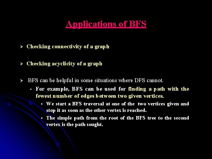
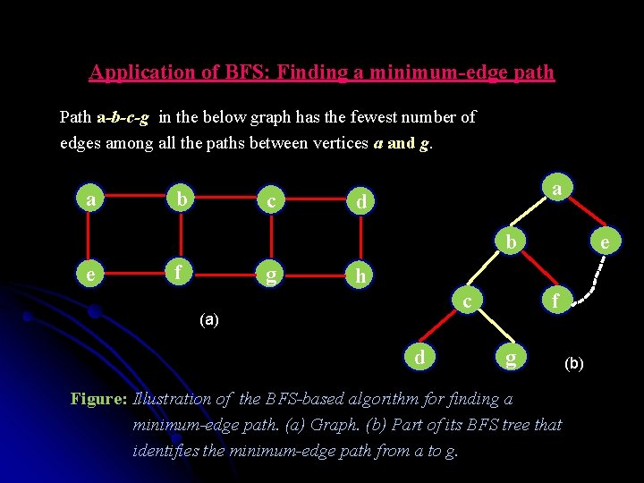
Applications of BFS Ø Checking connectivity of a graph Ø Checking acyclicity of a graph Ø BFS can be helpful in some situations where DFS cannot. • For example, BFS can be used for finding a path with the fewest number of edges between two given vertices. § § We start a BFS traversal at one of the two vertices given and stop it as soon as the other vertex is reached. The simple path from the root of the BFS tree to the second vertex is the path sought.

Application of BFS: Finding a minimum-edge path Path a-b-c-g in the below graph has the fewest number of edges among all the paths between vertices a and g. a b c a d b e f g e h c (a) d f g Figure: Illustration of the BFS-based algorithm for finding a minimum-edge path. (a) Graph. (b) Part of its BFS tree that identifies the minimum-edge path from a to g. (b)

Main facts about DFS and BFS DFS BFS Data structure stack queue No. of vertex orderings 2 orderings 1 ordering Edge types (undirected graphs) tree and back edges tree and cross edges Applications connectivity, acyclicity, articulation points minimum-edge paths Efficiency for adjacency matrix Θ(|V|2) Efficiency for adjacency lists Θ(|V| + |E|)

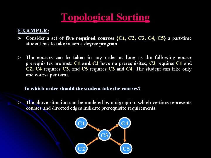
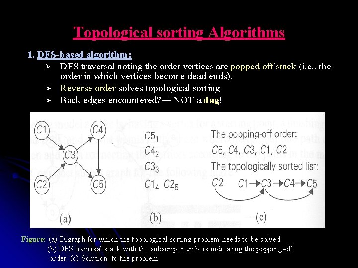
Topological Sorting EXAMPLE: Ø Consider a set of five required courses {C 1, C 2, C 3, C 4, C 5} a part-time student has to take in some degree program. Ø The courses can be taken in any order as long as the following course prerequisites are met: C 1 and C 2 have no prerequisites, C 3 requires C 1 and C 2, C 4 requires C 3, and C 5 requires C 3 and C 4. The student can take only one course per term. In which order should the student take the courses? Ø The above situation can be modeled by a digraph in which vertices represents courses and directed edges indicate prerequisite requirements. C 1 C 4 C 3 C 2 C 5

Topological Sorting Ø The question is whether we can list the vertices of a digraph in such an order that for every edge in the graph, the vertex where the edge starts is listed before the vertex where the edge ends. This problem is called topological sorting. Ø For topological sorting to be possible, a digraph must be a dag. i. e. , if a digraph has no cycles, the topological sorting problem for it has a solution. Ø There are two efficient algorithms that both verify whether a digraph is a dag, and if it is a dag then it produces an ordering of vertices that solves the topological sorting problem: § DFS – based algorithm § Source – removal algorithm

Topological sorting Algorithms 1. DFS-based algorithm: Ø DFS traversal noting the order vertices are popped off stack (i. e. , the order in which vertices become dead ends). Ø Reverse order solves topological sorting Ø Back edges encountered? → NOT a dag! Figure: (a) Digraph for which the topological sorting problem needs to be solved. (b) DFS traversal stack with the subscript numbers indicating the popping-off order. (c) Solution to the problem.

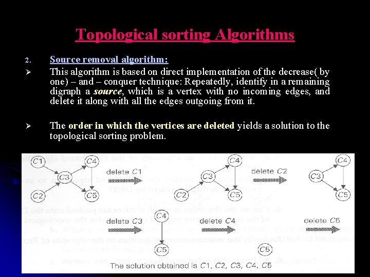
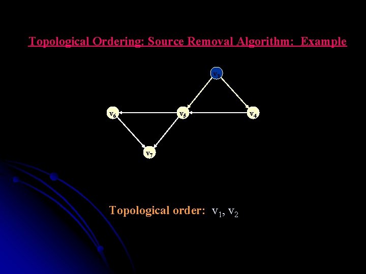
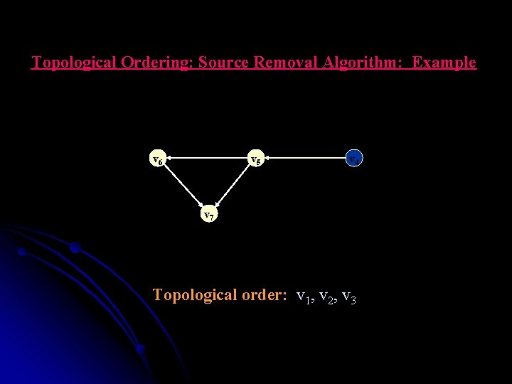
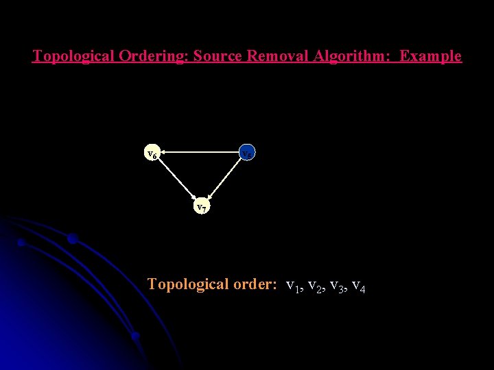
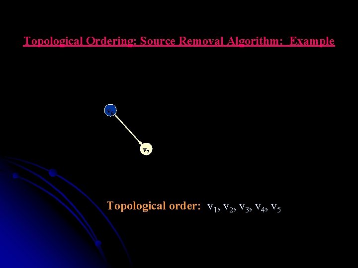
Topological sorting Algorithms 2. Ø Ø Source removal algorithm: This algorithm is based on direct implementation of the decrease( by one) – and – conquer technique: Repeatedly, identify in a remaining digraph a source, which is a vertex with no incoming edges, and delete it along with all the edges outgoing from it. The order in which the vertices are deleted yields a solution to the topological sorting problem. 68

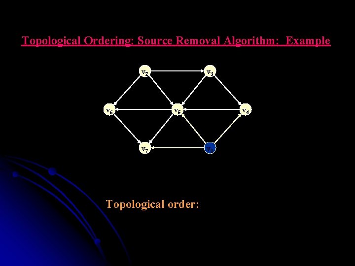
Topological Ordering: Source Removal Algorithm: Example v 2 v 6 v 3 v 5 v 7 Topological order: v 4 v 11

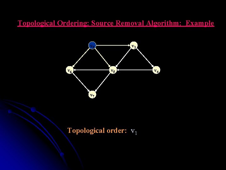
Topological Ordering: Source Removal Algorithm: Example v 22 v 6 v 3 v 5 v 7 Topological order: v 1 v 4

Topological Ordering: Source Removal Algorithm: Example v 33 v 6 v 5 v 7 Topological order: v 1, v 2 v 4

Topological Ordering: Source Removal Algorithm: Example v 6 v 5 v 44 v 7 Topological order: v 1, v 2, v 3

Topological Ordering: Source Removal Algorithm: Example v 55 v 6 v 7 Topological order: v 1, v 2, v 3, v 4

Topological Ordering: Source Removal Algorithm: Example v 66 v 7 Topological order: v 1, v 2, v 3, v 4, v 5

Topological Ordering: Source Removal Algorithm: Example v 77 Topological order: v 1, v 2, v 3, v 4, v 5, v 6

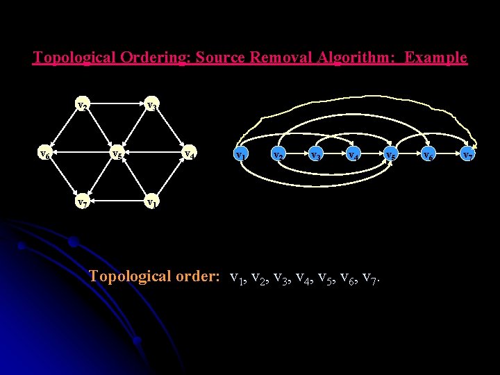
Topological Ordering: Source Removal Algorithm: Example v 2 v 6 v 3 v 5 v 7 v 4 v 1 v 2 v 3 v 4 v 1 Topological order: v 1, v 2, v 3, v 4, v 5, v 6, v 7. v 5 v 6 v 7

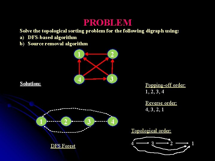
PROBLEM Solve the topological sorting problem for the following digraph using: a) DFS-based algorithm b) Source removal algorithm Solution: 1 2 4 3 Popping-off order: 1, 2, 3, 4 Reverse order: 4, 3, 2, 1 1 2 3 4 Topological order: DFS Forest 4 3 2 1

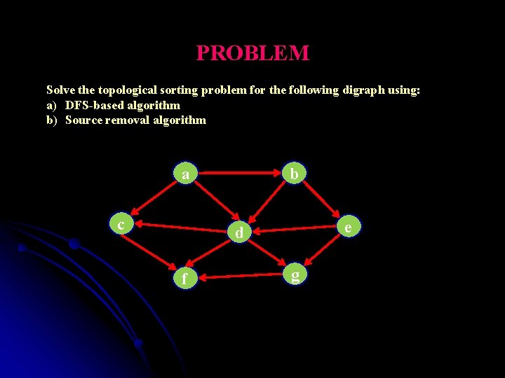
PROBLEM Solve the topological sorting problem for the following digraph using: a) DFS-based algorithm b) Source removal algorithm b a c e d f g

Algorithms for Generating Combinatorial Objects Ø Most important types of combinatorial objects are: l permutations l combinations l subsets of a given set Ø They typically arise in problems that require a consideration of different choices. Ø Combinatorial objects are studied in a branch of discrete mathematics called combinatorics. § Ø Mathematicians are primarily interested in different counting formulas which tell us how many items need to be generated. Here, we concentrate on algorithms for generating combinatorial objects, not just counting them.

Generating Permutations Ø Bottom-up minimal change algorithm Ø Johnson-Trotter algorithm Ø Lexicographic ordering

Generating Permutations Ø For simplicity, we assume that the underlying set whose elements need to be permuted is simply the set of integers from 1 to n § They can be interpreted as indices of elements in an n-element set {a 1, …, an} Ø What would the decrease-by-one technique suggest for the problem of generating all n! permutations of {1, …, n}?

Generating Permutations Ø Approach : § The smaller-by-one problem is to generate all (n-1)! permutations § Assuming that the smaller problem is solved, we can get a solution to the larger one • by inserting n in each of the n possible positions among elements of every permutation of n-1 elements. • There are two possible order of insertions: either left to right or right to left. § Total number of all permutations will be n. (n-1) ! = n!. Hence, we will obtain all the permutations of {1, …, n}.

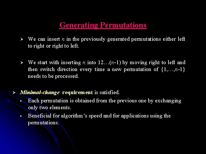
Generating Permutations Ø Ø We can insert n in the previously generated permutations either left to right or right to left. Ø We start with inserting n into 12…(n-1) by moving right to left and then switch direction every time a new permutation of {1, …, n-1} needs to be processed. Minimal-change requirement is satisfied. § Each permutation is obtained from the previous one by exchanging only two elements. § Beneficial for algorithm’s speed and for applications using the permutations.

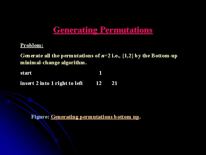
Generating Permutations Problem: Generate all the permutations of n=2 i. e. , {1, 2} by the Bottom-up minimal-change algorithm. start insert 2 into 1 right to left 1 12 21 Figure: Generating permutations bottom up.

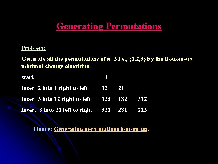
Generating Permutations Problem: Generate all the permutations of n=3 i. e. , {1, 2, 3} by the Bottom-up minimal-change algorithm. start 1 insert 2 into 1 right to left 12 21 insert 3 into 12 right to left 123 132 312 insert 3 into 21 left to right 321 231 213 Figure: Generating permutations bottom up.

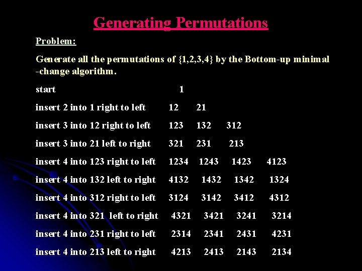
Generating Permutations Problem: Generate all the permutations of {1, 2, 3, 4} by the Bottom-up minimal -change algorithm. start 1 insert 2 into 1 right to left 12 21 insert 3 into 12 right to left 123 132 312 insert 3 into 21 left to right 321 231 213 insert 4 into 123 right to left 1234 1243 1423 4123 insert 4 into 132 left to right 4132 1432 1342 1324 insert 4 into 312 right to left 3124 3142 3412 4312 insert 4 into 321 left to right 4321 3421 3241 3214 insert 4 into 231 right to left 2314 2341 2431 4231 insert 4 into 213 left to right 4213 2413 2143 2134

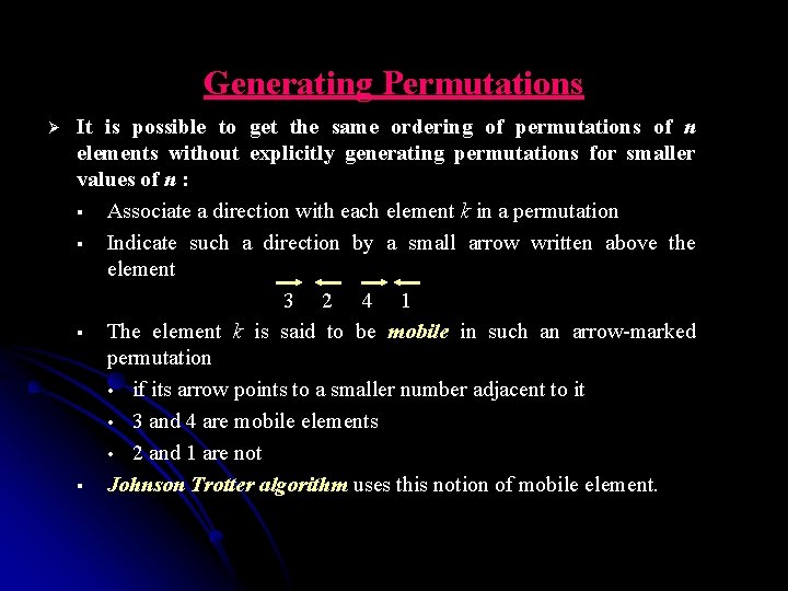
Generating Permutations Ø It is possible to get the same ordering of permutations of n elements without explicitly generating permutations for smaller values of n : § Associate a direction with each element k in a permutation § Indicate such a direction by a small arrow written above the element 3 2 4 1 § The element k is said to be mobile in such an arrow-marked permutation • if its arrow points to a smaller number adjacent to it • 3 and 4 are mobile elements • 2 and 1 are not § Johnson Trotter algorithm uses this notion of mobile element.

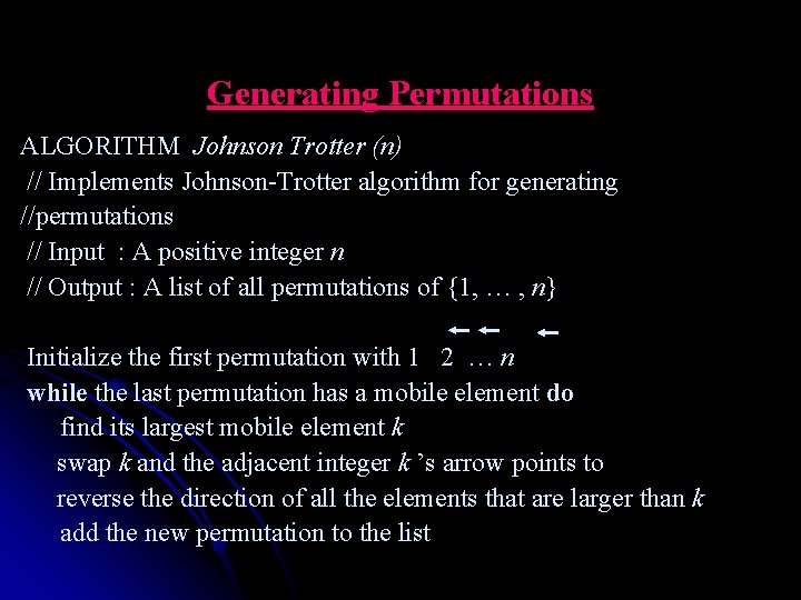
Generating Permutations ALGORITHM Johnson Trotter (n) // Implements Johnson-Trotter algorithm for generating //permutations // Input : A positive integer n // Output : A list of all permutations of {1, … , n} Initialize the first permutation with 1 2 … n while the last permutation has a mobile element do find its largest mobile element k swap k and the adjacent integer k ’s arrow points to reverse the direction of all the elements that are larger than k add the new permutation to the list

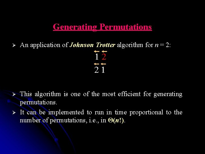
Generating Permutations Ø An application of Johnson Trotter algorithm for n = 2: 1 2 2 1 Ø Ø This algorithm is one of the most efficient for generating permutations. It can be implemented to run in time proportional to the number of permutations, i. e. , in Θ(n!).

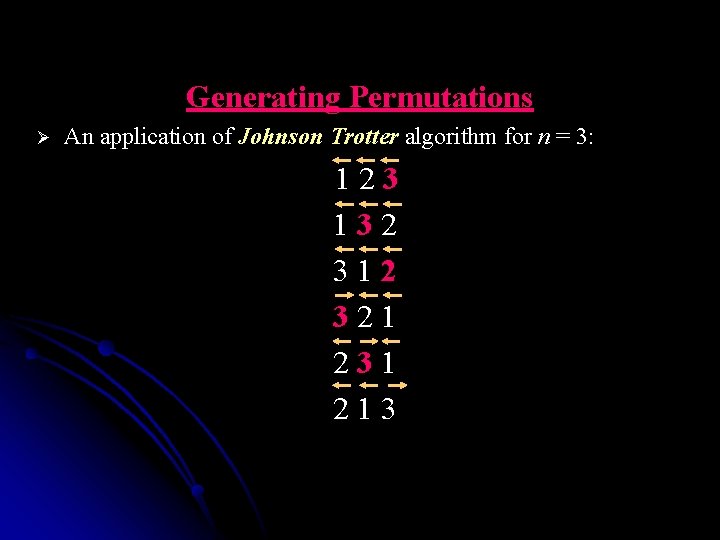
Generating Permutations Ø An application of Johnson Trotter algorithm for n = 3: 1 2 3 1 3 2 3 1 2 3 2 1 2 3 1 2 1 3

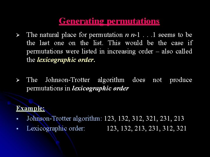
Generating permutations Ø The natural place for permutation n n-1. . . 1 seems to be the last one on the list. This would be the case if permutations were listed in increasing order – also called the lexicographic order. Ø The Johnson-Trotter algorithm does not produce permutations in lexicographic order Example: § Johnson-Trotter algorithm: 123, 132, 312, 321, 231, 213 § Lexicographic order: 123, 132, 213, 231, 312, 321

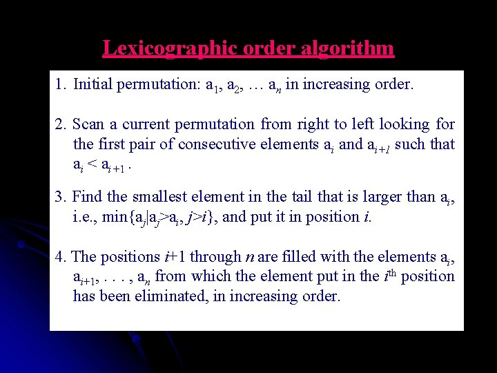
Lexicographic order algorithm 1. Initial permutation: a 1, a 2, … an in increasing order. 2. Scan a current permutation from right to left looking for the first pair of consecutive elements ai and ai+1 such that ai < ai+1. 3. Find the smallest element in the tail that is larger than ai, i. e. , min{aj|aj>ai, j>i}, and put it in position i. 4. The positions i+1 through n are filled with the elements ai, ai+1, . . . , an from which the element put in the ith position has been eliminated, in increasing order.

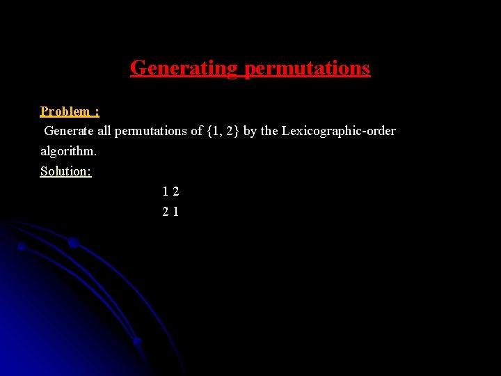
Generating permutations Problem : Generate all permutations of {1, 2} by the Lexicographic-order algorithm. Solution: 1 2 2 1

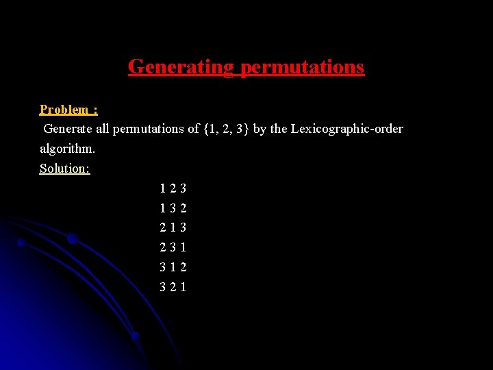
Generating permutations Problem : Generate all permutations of {1, 2, 3} by the Lexicographic-order algorithm. Solution: 1 2 3 1 3 2 2 1 3 2 3 1 3 1 2 3 2 1

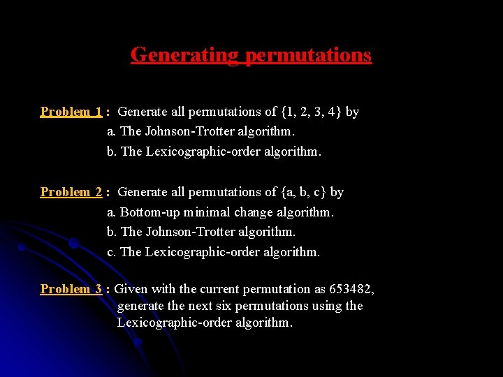
Generating permutations Problem 1 : Generate all permutations of {1, 2, 3, 4} by a. The Johnson-Trotter algorithm. b. The Lexicographic-order algorithm. Problem 2 : Generate all permutations of {a, b, c} by a. Bottom-up minimal change algorithm. b. The Johnson-Trotter algorithm. c. The Lexicographic-order algorithm. Problem 3 : Given with the current permutation as 653482, generate the next six permutations using the Lexicographic-order algorithm.

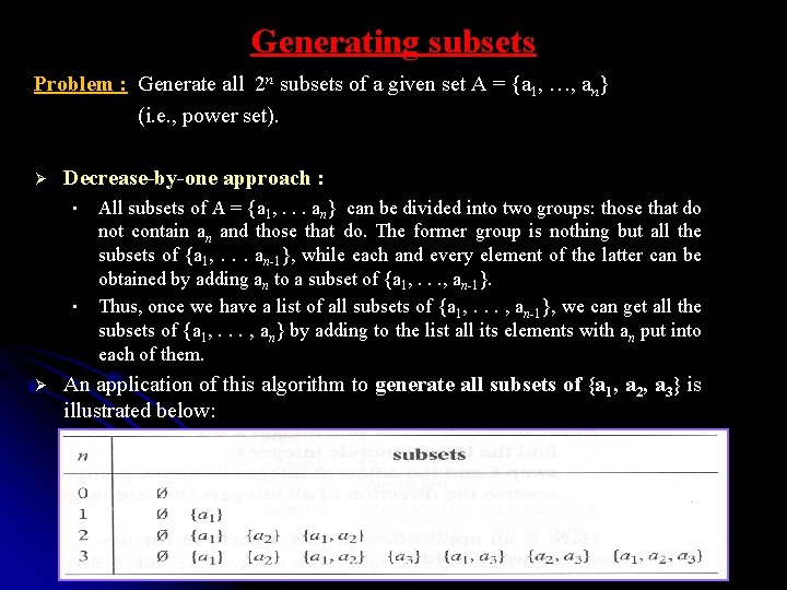
Generating subsets Problem : Generate all 2 n subsets of a given set A = {a 1, …, an} (i. e. , power set). Ø Decrease-by-one approach : • • Ø All subsets of A = {a 1, . . . an} can be divided into two groups: those that do not contain an and those that do. The former group is nothing but all the subsets of {a 1, . . . an-1}, while each and every element of the latter can be obtained by adding an to a subset of {a 1, . . . , an-1}. Thus, once we have a list of all subsets of {a 1, . . . , an-1}, we can get all the subsets of {a 1, . . . , an} by adding to the list all its elements with an put into each of them. An application of this algorithm to generate all subsets of {a 1, a 2, a 3} is illustrated below:

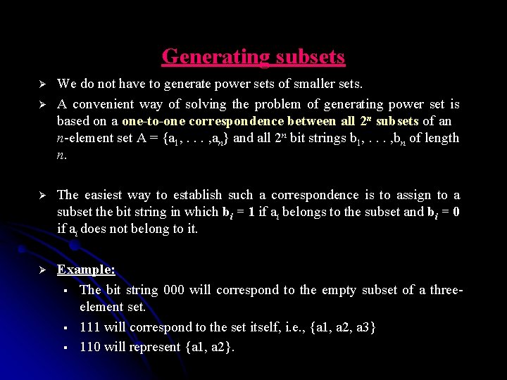
Generating subsets Ø Ø We do not have to generate power sets of smaller sets. A convenient way of solving the problem of generating power set is based on a one-to-one correspondence between all 2 n subsets of an n-element set A = {a 1, . . . , an} and all 2 n bit strings b 1, . . . , bn of length n. Ø The easiest way to establish such a correspondence is to assign to a subset the bit string in which bi = 1 if ai belongs to the subset and bi = 0 if ai does not belong to it. Ø Example: § The bit string 000 will correspond to the empty subset of a threeelement set. § 111 will correspond to the set itself, i. e. , {a 1, a 2, a 3} § 110 will represent {a 1, a 2}.

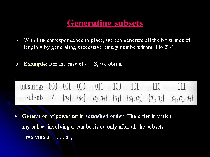
Generating subsets Ø With this correspondence in place, we can generate all the bit strings of length n by generating successive binary numbers from 0 to 2 n-1. Ø Example: For the case of n = 3, we obtain Ø Generation of power set in squashed order: The order in which any subset involving aj can be listed only after all the subsets involving a 1, . . . , aj-1.

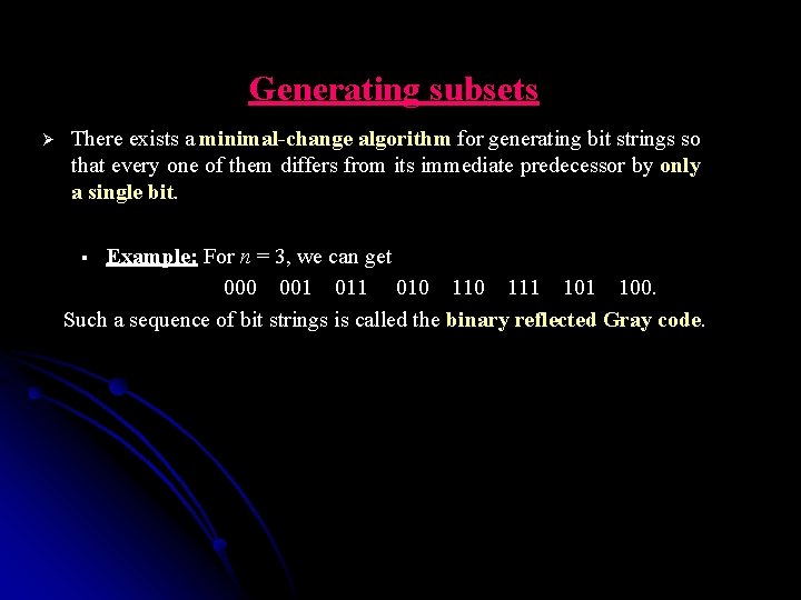
Generating subsets Ø There exists a minimal-change algorithm for generating bit strings so that every one of them differs from its immediate predecessor by only a single bit. Example: For n = 3, we can get 000 001 011 010 111 100. Such a sequence of bit strings is called the binary reflected Gray code. §

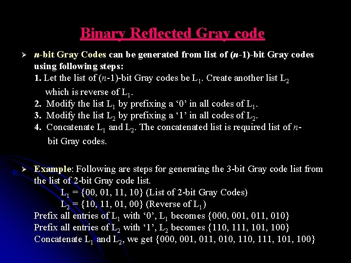
Binary Reflected Gray code n-bit Gray Codes can be generated from list of (n-1)-bit Gray codes using following steps: 1. Let the list of (n-1)-bit Gray codes be L 1. Create another list L 2 which is reverse of L 1. 2. Modify the list L 1 by prefixing a ‘ 0’ in all codes of L 1. 3. Modify the list L 2 by prefixing a ‘ 1’ in all codes of L 2. 4. Concatenate L 1 and L 2. The concatenated list is required list of n bit Gray codes. Ø Ø Example: Following are steps for generating the 3 -bit Gray code list from the list of 2 -bit Gray code list. L 1 = {00, 01, 10} (List of 2 -bit Gray Codes) L 2 = {10, 11, 00} (Reverse of L 1) Prefix all entries of L 1 with ‘ 0’, L 1 becomes {000, 001, 010} Prefix all entries of L 2 with ‘ 1’, L 2 becomes {110, 111, 100} Concatenate L 1 and L 2, we get {000, 001, 010, 111, 100}

End of Chapter 5