Algorithms for SELECT and JOIN Operations 8 n

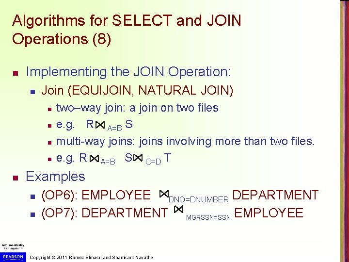
Algorithms for SELECT and JOIN Operations (8) n Implementing the JOIN Operation: n Join (EQUIJOIN, NATURAL JOIN) n n n two–way join: a join on two files e. g. R A=B S multi-way joins: joins involving more than two files. e. g. R A=B S C=D T Examples n n (OP 6): EMPLOYEE DNO=DNUMBER DEPARTMENT (OP 7): DEPARTMENT MGRSSN=SSN EMPLOYEE Copyright © 2011 Ramez Elmasri and Shamkant Navathe

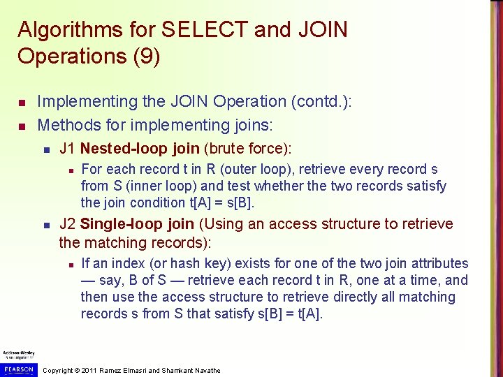
Algorithms for SELECT and JOIN Operations (9) n n Implementing the JOIN Operation (contd. ): Methods for implementing joins: n J 1 Nested-loop join (brute force): n n For each record t in R (outer loop), retrieve every record s from S (inner loop) and test whether the two records satisfy the join condition t[A] = s[B]. J 2 Single-loop join (Using an access structure to retrieve the matching records): n If an index (or hash key) exists for one of the two join attributes — say, B of S — retrieve each record t in R, one at a time, and then use the access structure to retrieve directly all matching records s from S that satisfy s[B] = t[A]. Copyright © 2011 Ramez Elmasri and Shamkant Navathe

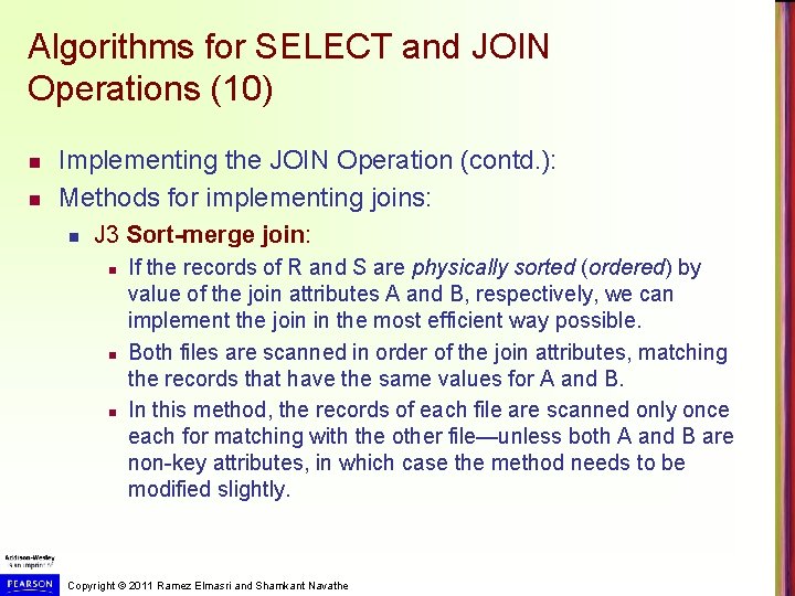
Algorithms for SELECT and JOIN Operations (10) n n Implementing the JOIN Operation (contd. ): Methods for implementing joins: n J 3 Sort-merge join: n n n If the records of R and S are physically sorted (ordered) by value of the join attributes A and B, respectively, we can implement the join in the most efficient way possible. Both files are scanned in order of the join attributes, matching the records that have the same values for A and B. In this method, the records of each file are scanned only once each for matching with the other file—unless both A and B are non-key attributes, in which case the method needs to be modified slightly. Copyright © 2011 Ramez Elmasri and Shamkant Navathe

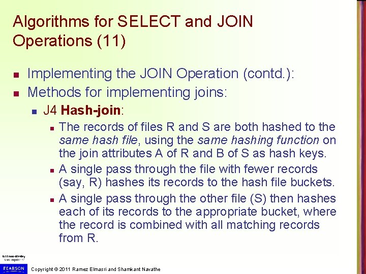
Algorithms for SELECT and JOIN Operations (11) n n Implementing the JOIN Operation (contd. ): Methods for implementing joins: n J 4 Hash-join: n n n The records of files R and S are both hashed to the same hash file, using the same hashing function on the join attributes A of R and B of S as hash keys. A single pass through the file with fewer records (say, R) hashes its records to the hash file buckets. A single pass through the other file (S) then hashes each of its records to the appropriate bucket, where the record is combined with all matching records from R. Copyright © 2011 Ramez Elmasri and Shamkant Navathe

Join Operation Copyright © 2011 Ramez Elmasri and Shamkant Navathe

Algorithms for SELECT and JOIN Operations (14) n n Implementing the JOIN Operation (contd. ): Factors affecting JOIN performance n n n Available buffer space Join selection factor Choice of inner VS outer relation Copyright © 2011 Ramez Elmasri and Shamkant Navathe

Algorithms for SELECT and JOIN Operations (15) n n n Implementing the JOIN Operation (contd. ): Other types of JOIN algorithms Partition hash join n Partitioning phase: n Each file (R and S) is first partitioned into M partitions using a partitioning hash function on the join attributes: n n R 1 , R 2 , R 3 , . . . Rm and S 1 , S 2 , S 3 , . . . Sm Minimum number of in-memory buffers needed for the partitioning phase: M+1. A disk sub-file is created per partition to store the tuples for that partition. Joining or probing phase: n n Involves M iterations, one per partitioned file. Iteration i involves joining partitions Ri and Si. Copyright © 2011 Ramez Elmasri and Shamkant Navathe

Algorithms for SELECT and JOIN Operations (16) n n Implementing the JOIN Operation (contd. ): Partitioned Hash Join Procedure: n Assume Ri is smaller than Si. 1. Copy records from Ri into memory buffers. 2. Read all blocks from Si, one at a time and each record from Si is used to probe for a matching record(s) from partition Si. 3. Write matching record from Ri after joining to the record from Si into the result file. Copyright © 2011 Ramez Elmasri and Shamkant Navathe

Algorithms for SELECT and JOIN Operations (17) n n Implementing the JOIN Operation (contd. ): Cost analysis of partition hash join: 1. Reading and writing each record from R and S during the partitioning phase: (b. R + b. S), (b. R + b. S) 2. Reading each record during the joining phase: (b. R + b. S) 3. Writing the result of join: b. RES n Total Cost: n 3* (b. R + b. S) + b. RES Copyright © 2011 Ramez Elmasri and Shamkant Navathe

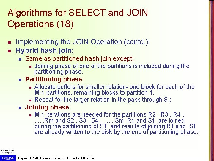
Algorithms for SELECT and JOIN Operations (18) n n Implementing the JOIN Operation (contd. ): Hybrid hash join: n Same as partitioned hash join except: n n Partitioning phase: n n n Joining phase of one of the partitions is included during the partitioning phase. Allocate buffers for smaller relation- one block for each of the M-1 partitions, remaining blocks to partition 1. Repeat for the larger relation in the pass through S. ) Joining phase: n M-1 iterations are needed for the partitions R 2 , R 3 , R 4 , . . . Rm and S 2 , S 3 , S 4 , . . . Sm. R 1 and S 1 are joined during the partitioning of S 1, and results of joining R 1 and S 1 are already written to the disk by the end of partitioning phase. Copyright © 2011 Ramez Elmasri and Shamkant Navathe

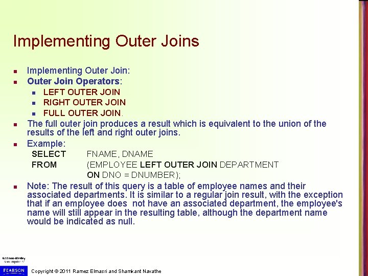
Implementing Outer Joins n n Implementing Outer Join: Outer Join Operators: n n n LEFT OUTER JOIN RIGHT OUTER JOIN FULL OUTER JOIN. The full outer join produces a result which is equivalent to the union of the results of the left and right outer joins. Example: SELECT FROM n FNAME, DNAME (EMPLOYEE LEFT OUTER JOIN DEPARTMENT ON DNO = DNUMBER); Note: The result of this query is a table of employee names and their associated departments. It is similar to a regular join result, with the exception that if an employee does not have an associated department, the employee's name will still appear in the resulting table, although the department name would be indicated as null. Copyright © 2011 Ramez Elmasri and Shamkant Navathe

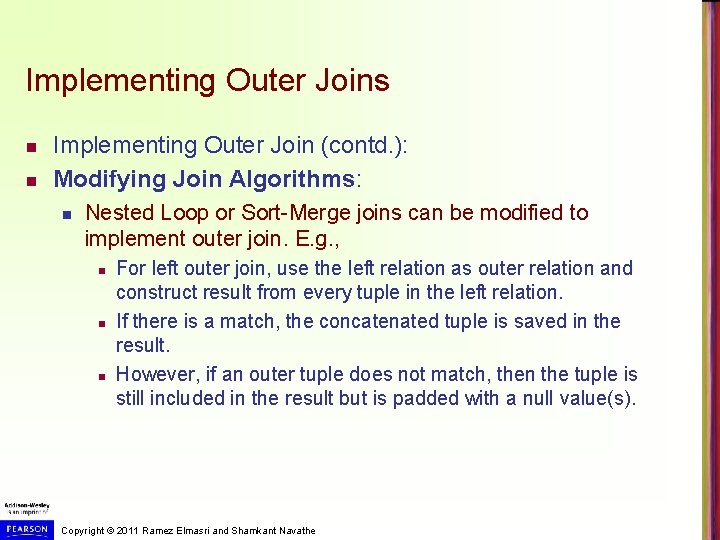
Implementing Outer Joins n n Implementing Outer Join (contd. ): Modifying Join Algorithms: n Nested Loop or Sort-Merge joins can be modified to implement outer join. E. g. , n n n For left outer join, use the left relation as outer relation and construct result from every tuple in the left relation. If there is a match, the concatenated tuple is saved in the result. However, if an outer tuple does not match, then the tuple is still included in the result but is padded with a null value(s). Copyright © 2011 Ramez Elmasri and Shamkant Navathe

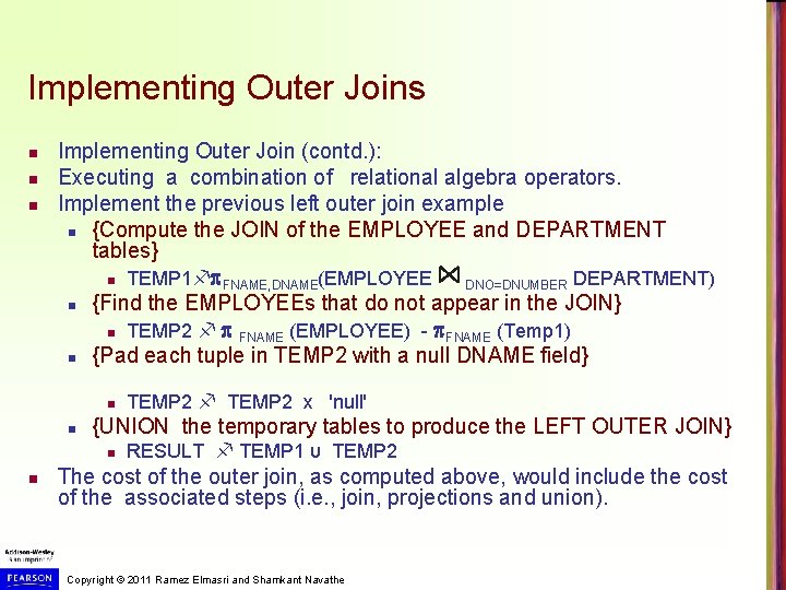
Implementing Outer Joins n n n Implementing Outer Join (contd. ): Executing a combination of relational algebra operators. Implement the previous left outer join example n {Compute the JOIN of the EMPLOYEE and DEPARTMENT tables} n TEMP 1 FNAME, DNAME(EMPLOYEE DNO=DNUMBER DEPARTMENT) n {Find the EMPLOYEEs that do not appear in the JOIN} n TEMP 2 FNAME (EMPLOYEE) - FNAME (Temp 1) n {Pad each tuple in TEMP 2 with a null DNAME field} n n {UNION the temporary tables to produce the LEFT OUTER JOIN} n n TEMP 2 x 'null' RESULT TEMP 1 υ TEMP 2 The cost of the outer join, as computed above, would include the cost of the associated steps (i. e. , join, projections and union). Copyright © 2011 Ramez Elmasri and Shamkant Navathe

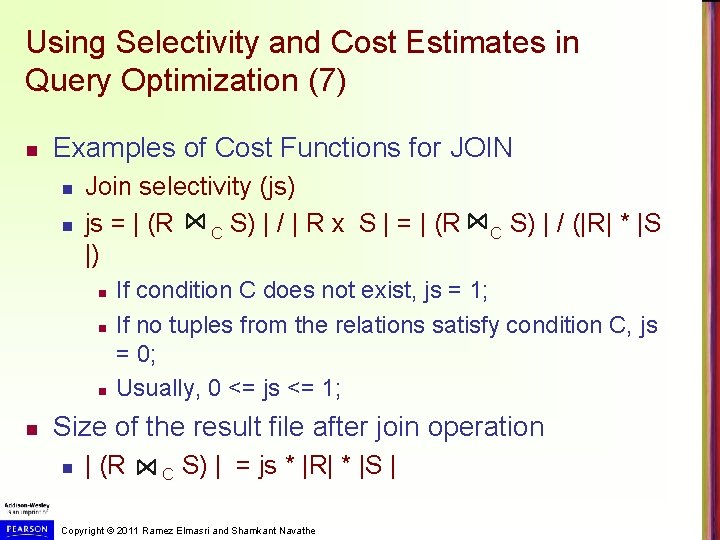
Using Selectivity and Cost Estimates in Query Optimization (7) n Examples of Cost Functions for JOIN n n Join selectivity (js) js = | (R C S) | / | R x S | = | (R C S) | / (|R| * |S |) n n If condition C does not exist, js = 1; If no tuples from the relations satisfy condition C, js = 0; Usually, 0 <= js <= 1; Size of the result file after join operation n | (R C S) | = js * |R| * |S | Copyright © 2011 Ramez Elmasri and Shamkant Navathe

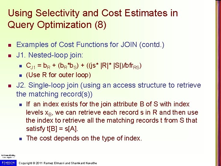
Using Selectivity and Cost Estimates in Query Optimization (8) n n Examples of Cost Functions for JOIN (contd. ) J 1. Nested-loop join: n n n CJ 1 = b. R + (b. R*b. S) + ((js* |R|* |S|)/bfr. RS) (Use R for outer loop) J 2. Single-loop join (using an access structure to retrieve the matching record(s)) n n If an index exists for the join attribute B of S with index levels x. B, we can retrieve each record s in R and then use the index to retrieve all the matching records t from S that satisfy t[B] = s[A]. The cost depends on the type of index. Copyright © 2011 Ramez Elmasri and Shamkant Navathe

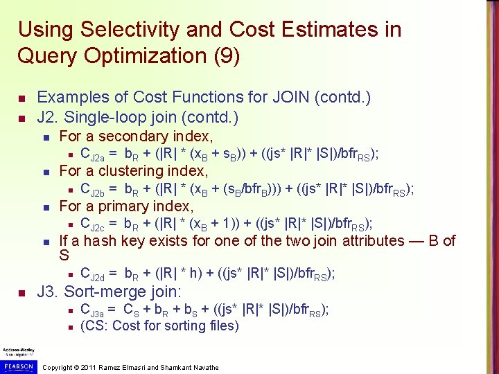
Using Selectivity and Cost Estimates in Query Optimization (9) n n Examples of Cost Functions for JOIN (contd. ) J 2. Single-loop join (contd. ) n For a secondary index, n n For a clustering index, n n CJ 2 c = b. R + (|R| * (x. B + 1)) + ((js* |R|* |S|)/bfr. RS); If a hash key exists for one of the two join attributes — B of S n n CJ 2 b = b. R + (|R| * (x. B + (s. B/bfr. B))) + ((js* |R|* |S|)/bfr. RS); For a primary index, n n CJ 2 a = b. R + (|R| * (x. B + s. B)) + ((js* |R|* |S|)/bfr. RS); CJ 2 d = b. R + (|R| * h) + ((js* |R|* |S|)/bfr. RS); J 3. Sort-merge join: n n CJ 3 a = CS + b. R + b. S + ((js* |R|* |S|)/bfr. RS); (CS: Cost for sorting files) Copyright © 2011 Ramez Elmasri and Shamkant Navathe

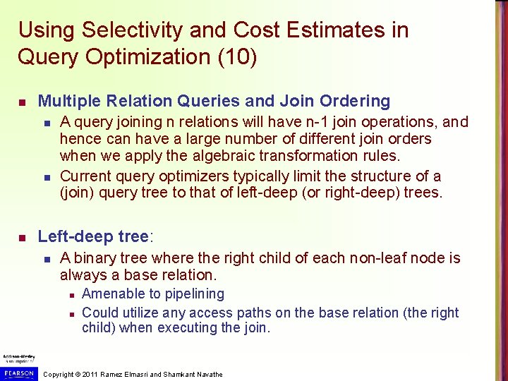
Using Selectivity and Cost Estimates in Query Optimization (10) n Multiple Relation Queries and Join Ordering n n n A query joining n relations will have n-1 join operations, and hence can have a large number of different join orders when we apply the algebraic transformation rules. Current query optimizers typically limit the structure of a (join) query tree to that of left-deep (or right-deep) trees. Left-deep tree: n A binary tree where the right child of each non-leaf node is always a base relation. n n Amenable to pipelining Could utilize any access paths on the base relation (the right child) when executing the join. Copyright © 2011 Ramez Elmasri and Shamkant Navathe