UnionFind A data structure for maintaining a collection

Union-Find A data structure for maintaining a collection of disjoint sets Course: Data Structures Lecturers: Haim Kaplan and Uri Zwick Last Updated: June 11, 2018

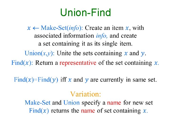
Union-Find •

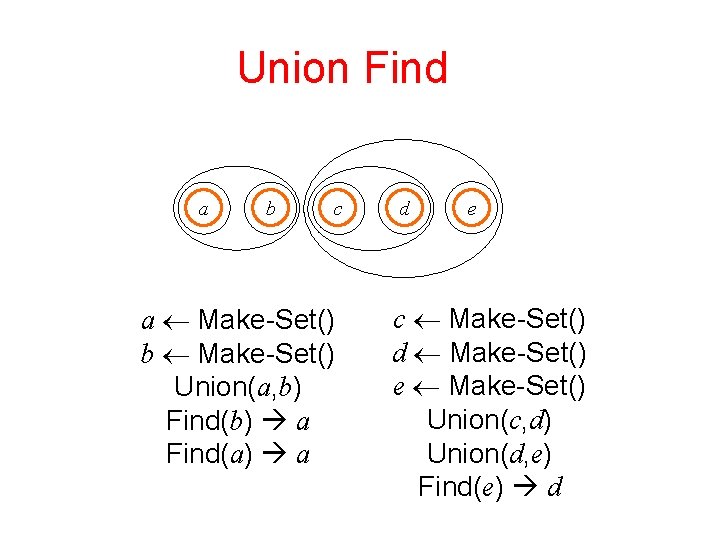
Union Find a b c a Make-Set() b Make-Set() Union(a, b) Find(b) a Find(a) a d e c Make-Set() d Make-Set() e Make-Set() Union(c, d) Union(d, e) Find(e) d

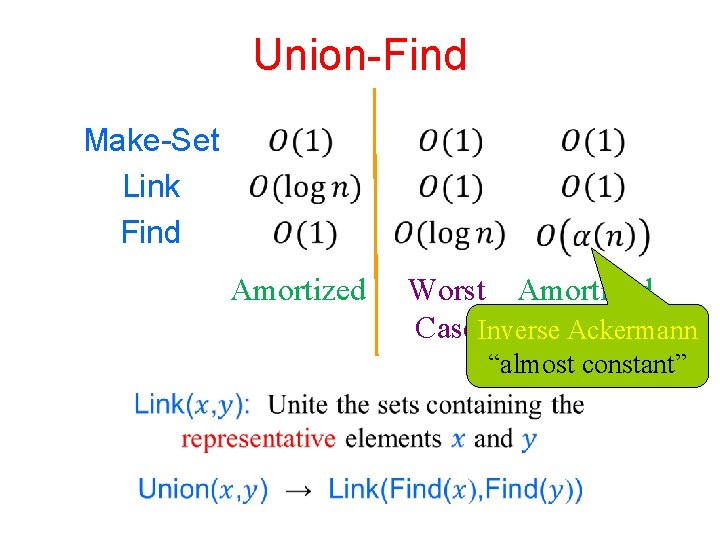
Union-Find Make-Set Link Find Amortized Worst Amortized Case. Inverse Ackermann “almost constant”

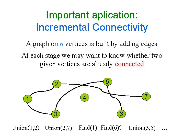
Important aplication: Incremental Connectivity A graph on n vertices is built by adding edges At each stage we may want to know whether two given vertices are already connected 5 2 7 4 1 3 Union(1, 2) Union(2, 7) 6 Find(1)=Find(6)? Union(3, 5) …

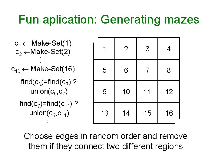
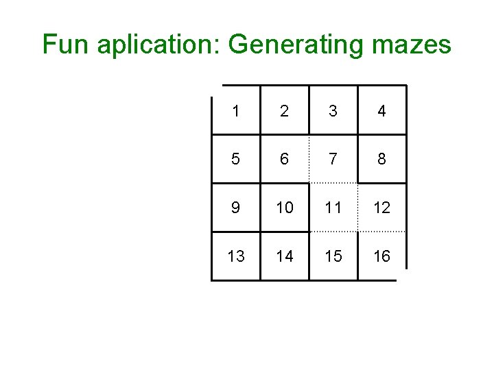
Fun aplication: Generating mazes 1 2 3 4 c 16 Make-Set(16) 5 6 7 8 find(c 6)=find(c 7) ? union(c 6, c 7) 9 10 11 12 find(c 7)=find(c 11) ? union(c 7, c 11) 13 14 15 16 … c 1 Make-Set(1) c 2 Make-Set(2) … Choose edges in random order and remove them if they connect two different regions

Fun aplication: Generating mazes 1 2 3 4 5 6 7 8 9 10 11 12 13 14 15 16

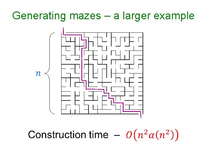
Generating mazes – a larger example

More serious aplications: • • Maintaining an equivalence relation Incremental connectivity in graphs Computing minimum spanning trees …

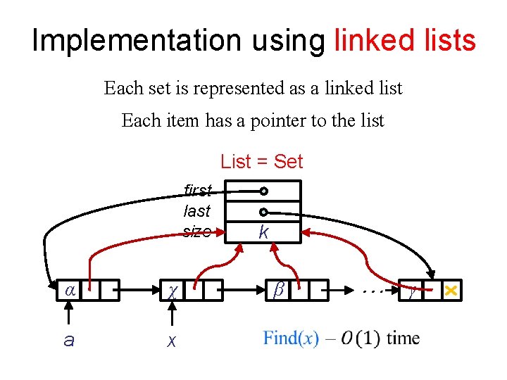
Implementation using linked lists Each set is represented as a linked list Each item has a pointer to the list List = Set first last size α χ a x k … β γ

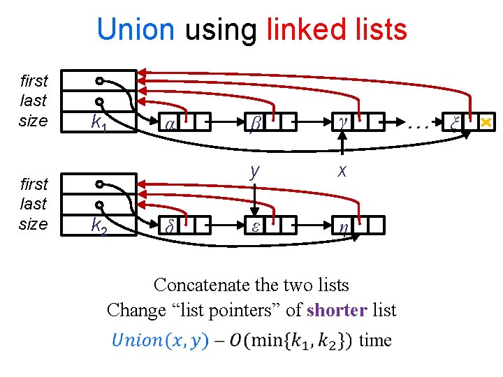
Union using linked lists first last size k 1 k 2 α δ β γ y x ε η Concatenate the two lists Change “list pointers” of shorter list … ξ

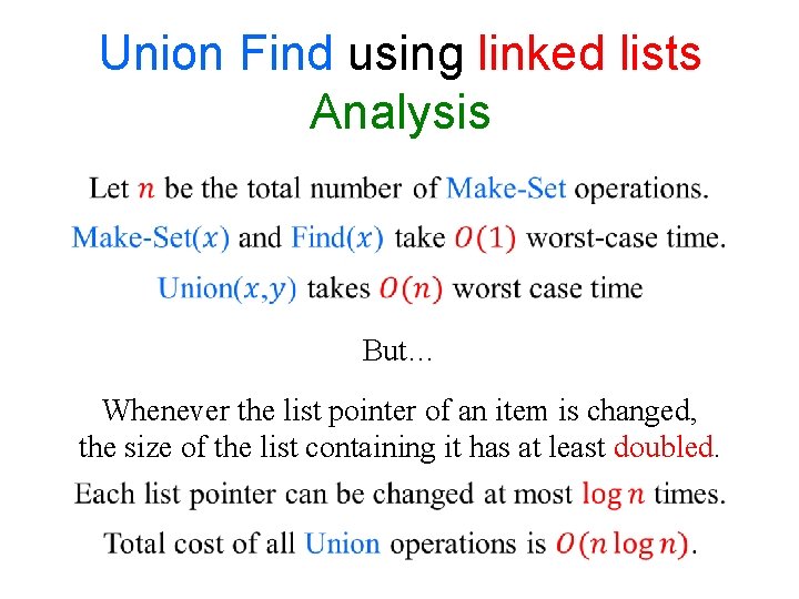
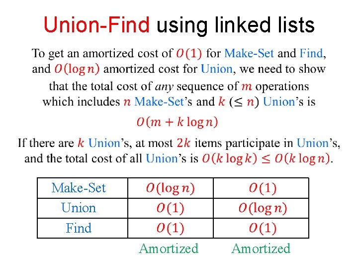
Union Find using linked lists Analysis But… Whenever the list pointer of an item is changed, the size of the list containing it has at least doubled.

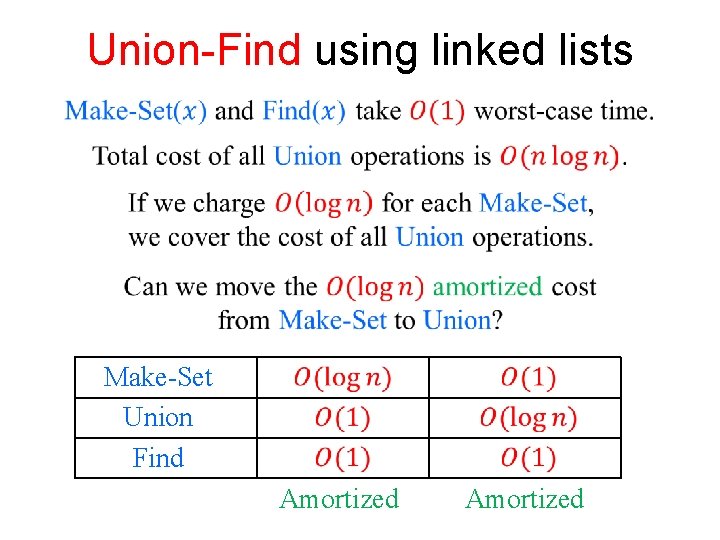
Union-Find using linked lists Make-Set Union Find Amortized

Union-Find using linked lists Make-Set Union Find Amortized

Union-Find Make-Set Link Find Amortized Worst Amortized Case. Inverse Ackermann “almost constant”

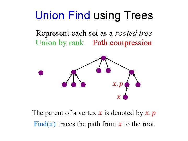
Union Find using Trees Represent each set as a rooted tree Union by rank Path compression

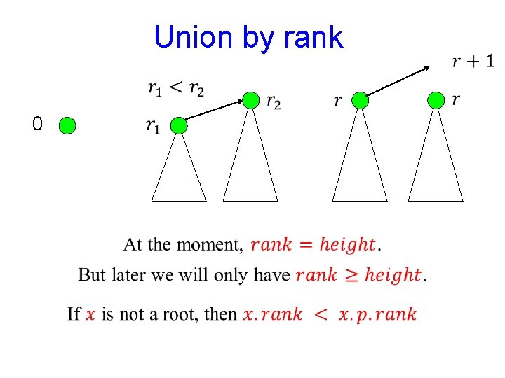
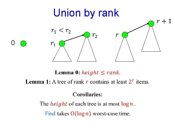
Union by rank 0

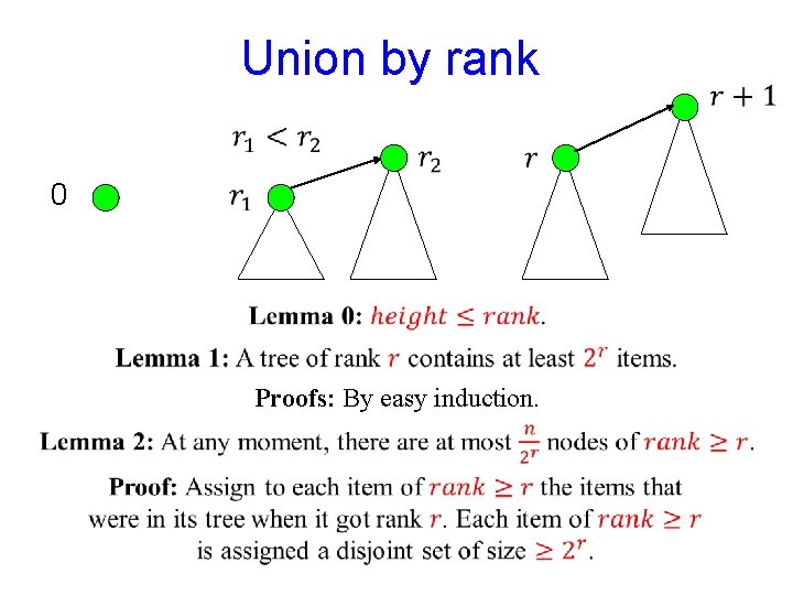
Union by rank 0 Proofs: By easy induction.

Union by rank 0 Corollaries:

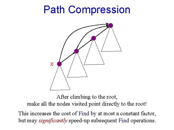
Path Compression After climbing to the root, make all the nodes visited point directly to the root! This increases the cost of Find by at most a constant factor, but may significantly speed-up subsequent Find operations.

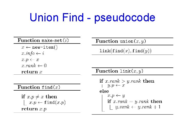
Union Find - pseudocode

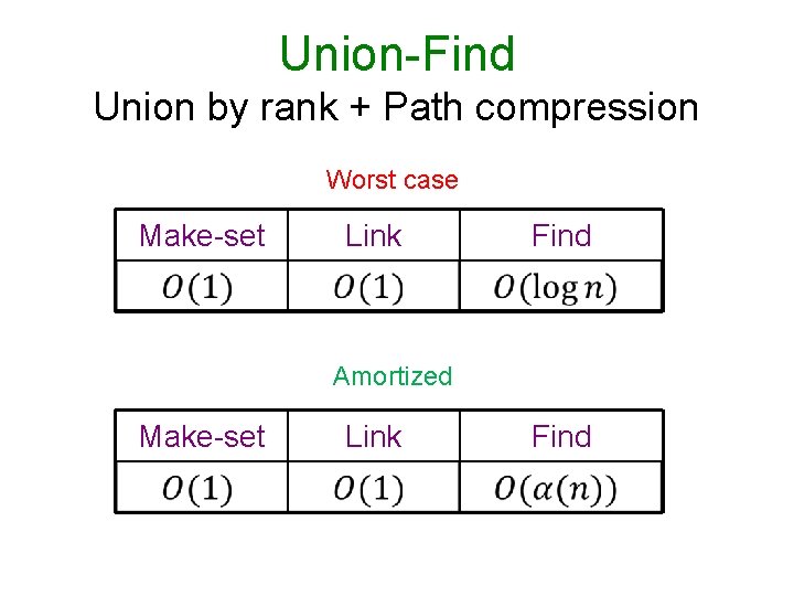
Union-Find Union by rank + Path compression Worst case Make-set Link Find Amortized Make-set Link Find

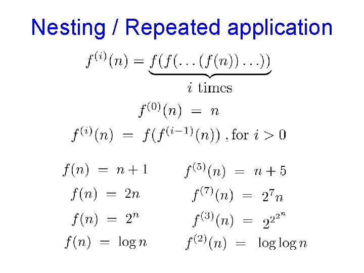
Nesting / Repeated application

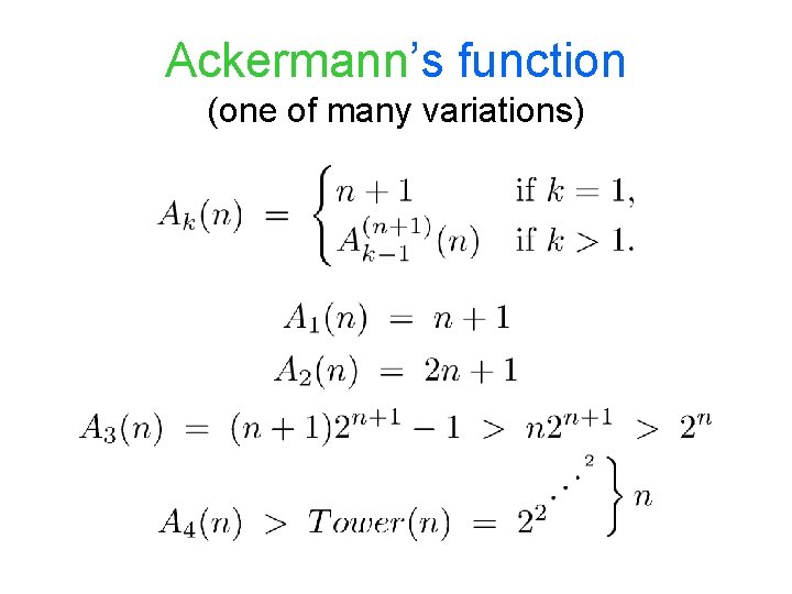
Ackermann’s function (one of many variations)

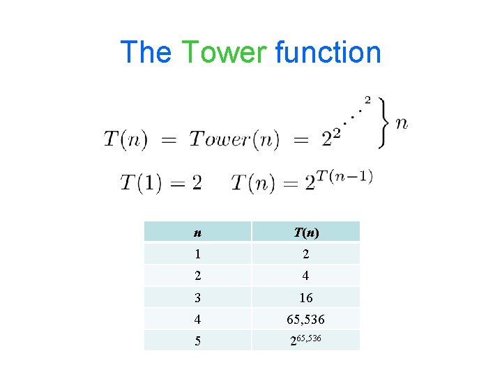
The Tower function n T(n) 1 2 2 4 3 16 4 65, 536 5 265, 536

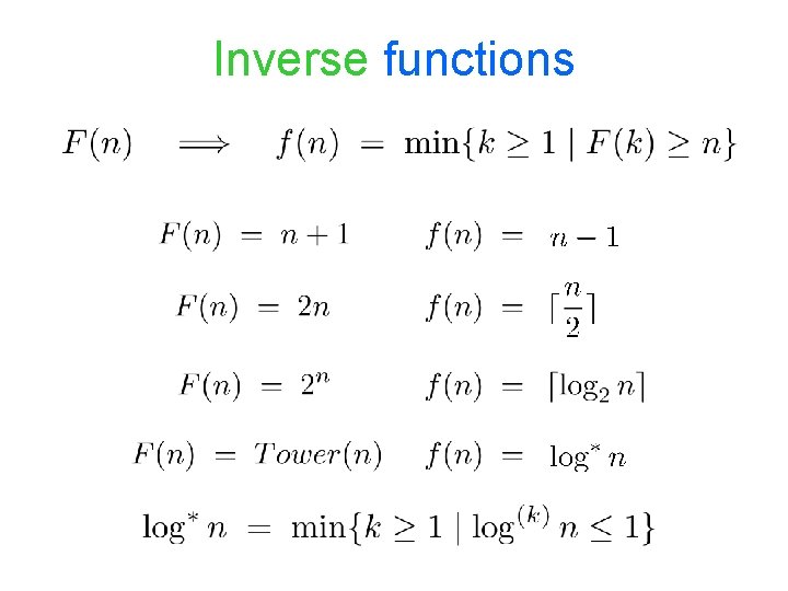
Inverse functions

n log*(n) [0, 2] [3, 4] [ 5 , 16 ] [ 17 , 65, 536 ] [ 65, 537 , 265, 536 ] 1 2 3 4 5

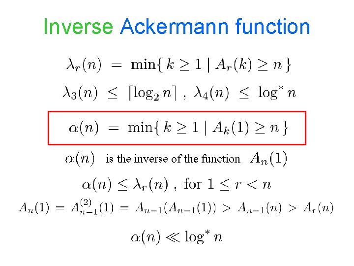
Inverse Ackermann function is the inverse of the function

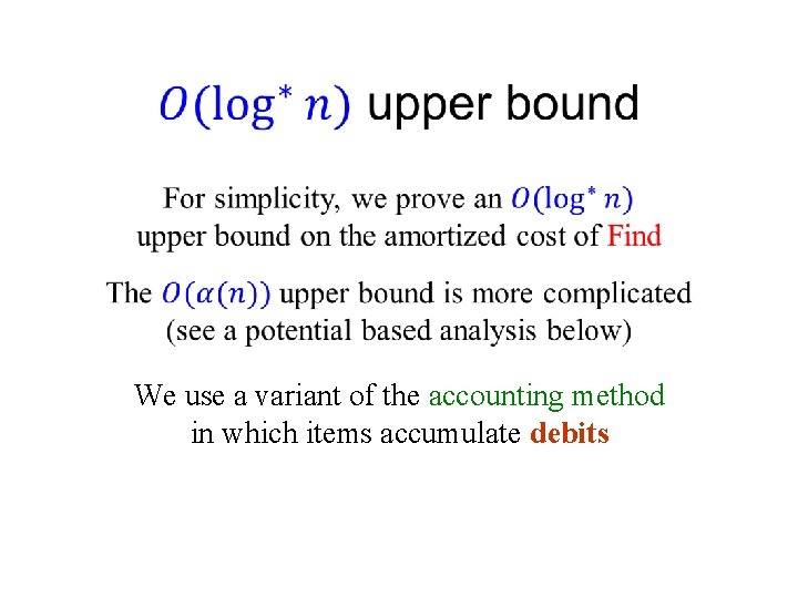
We use a variant of the accounting method in which items accumulate debits

[ 0 , 2 ] [ 3 , 4 ] [ 5 , 16 ] [ 17 , 65, 536 ] [ 65, 537 , 265, 536 ] 1 2 3 4 5

[ 0 , 2 ] The number of nodes of level 1

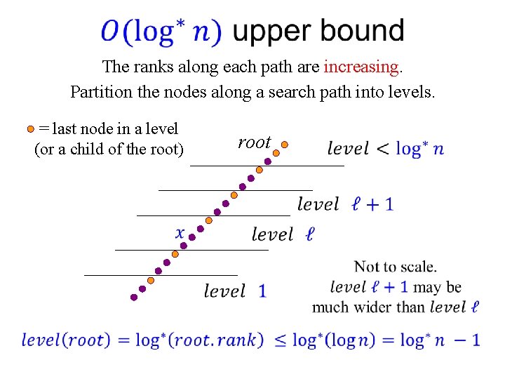
The ranks along each path are increasing. Partition the nodes along a search path into levels. = last node in a level (or a child of the root) root

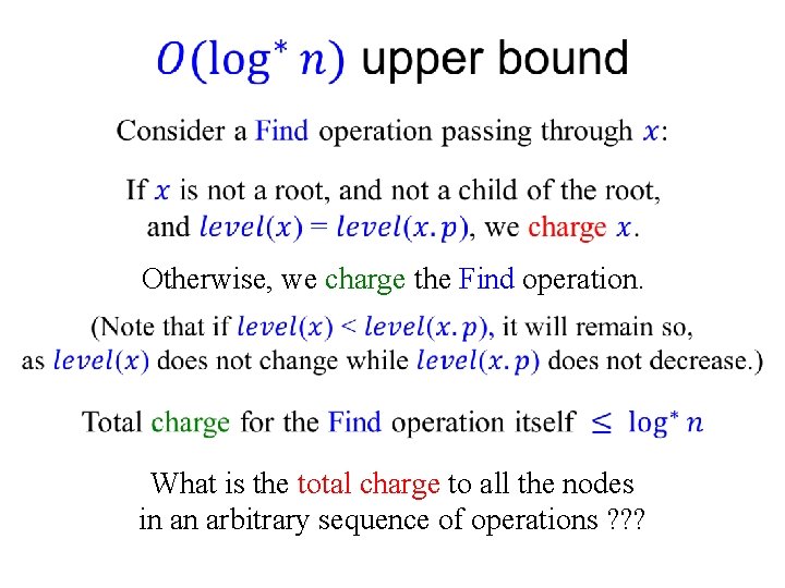
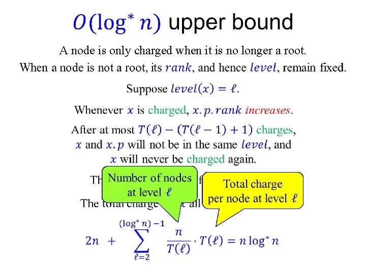
Otherwise, we charge the Find operation. What is the total charge to all the nodes in an arbitrary sequence of operations ? ? ?

A node is only charged when it is no longer a root.

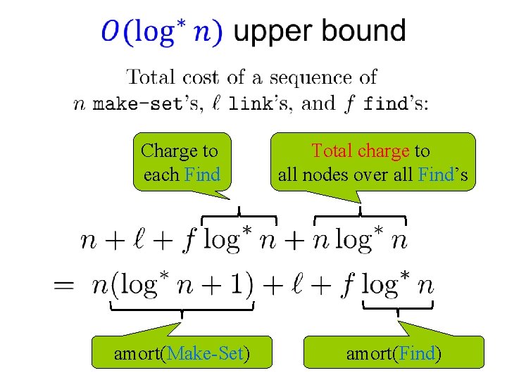
Charge to each Find amort(Make-Set) Total charge to all nodes over all Find’s amort(Find)

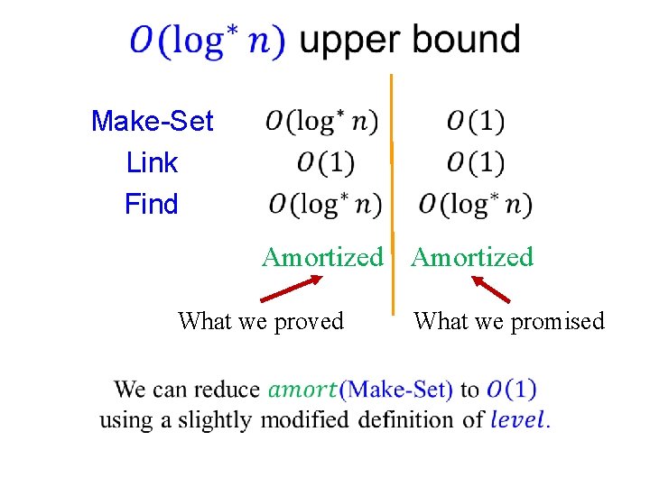
Make-Set Link Find Amortized What we proved What we promised

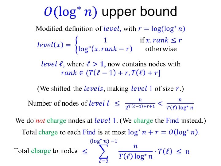
Total charge to nodes

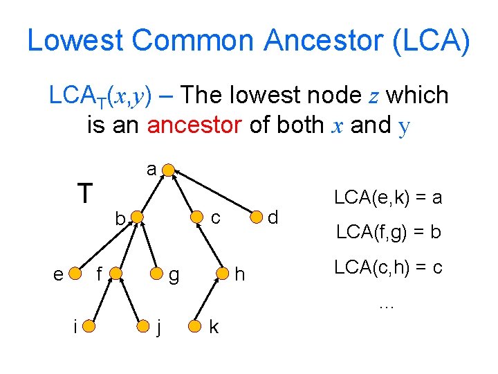
Lowest Common Ancestor (LCA) LCAT(x, y) – The lowest node z which is an ancestor of both x and y a T e c b f g d h LCA(e, k) = a LCA(f, g) = b LCA(c, h) = c … i j k

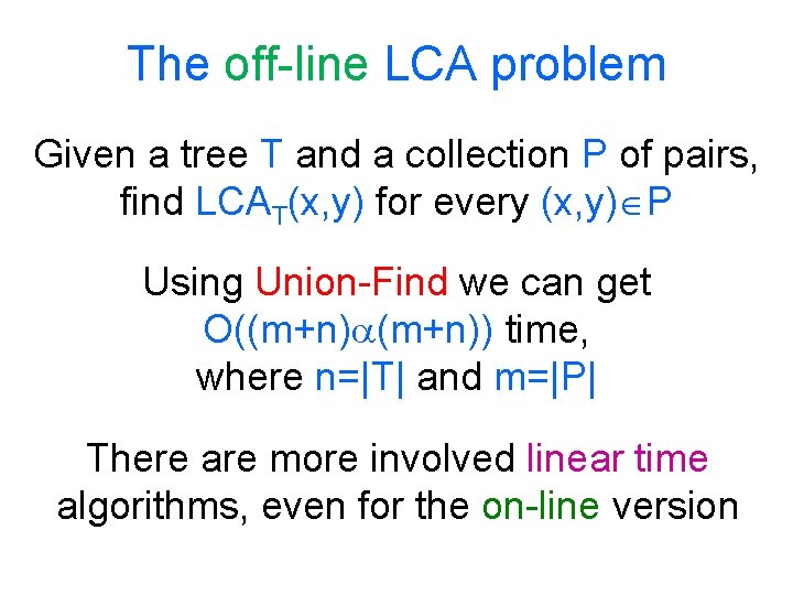
The off-line LCA problem Given a tree T and a collection P of pairs, find LCAT(x, y) for every (x, y) P Using Union-Find we can get O((m+n)) time, where n=|T| and m=|P| There are more involved linear time algorithms, even for the on-line version

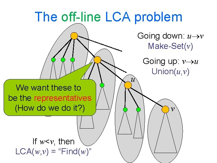
The off-line LCA problem Going down: u v Make-Set(v) We want these to be the representatives (How do we do it? ) If w<v, then LCA(w, v) = “Find(w)” u Going up: v u Union(u, v) v

The O( (n)) upper bound for Union-Find (For those interested)

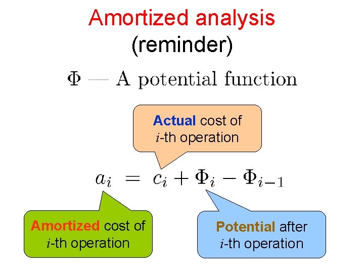
Amortized analysis (reminder) Actual cost of i-th operation Amortized cost of i-th operation Potential after i-th operation

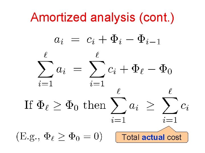
Amortized analysis (cont. ) Total actual cost

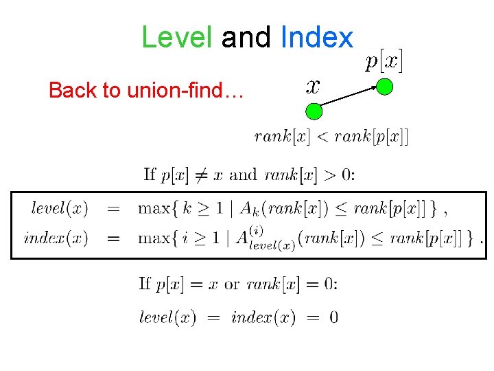
Level and Index Back to union-find…

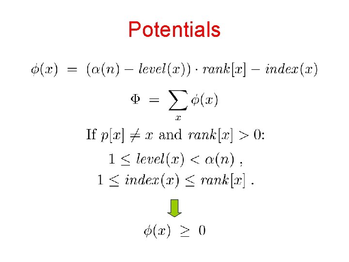
Potentials

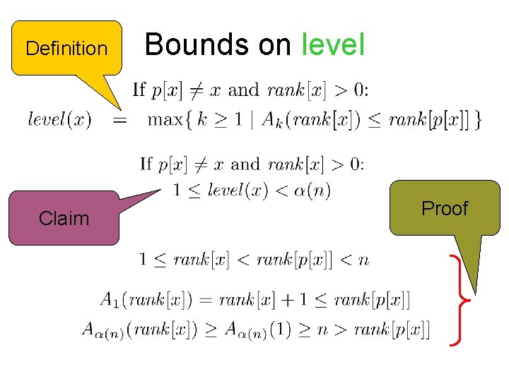
Definition Claim Bounds on level Proof

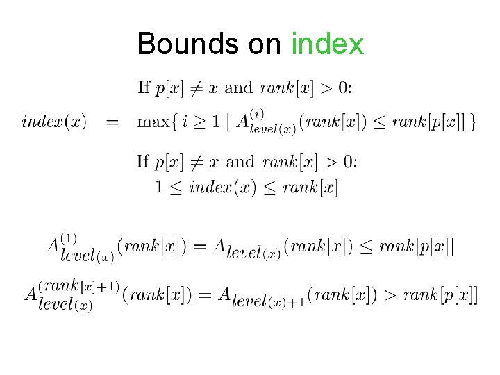
Bounds on index

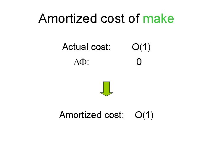
Amortized cost of make Actual cost: O(1) : 0 Amortized cost: O(1)

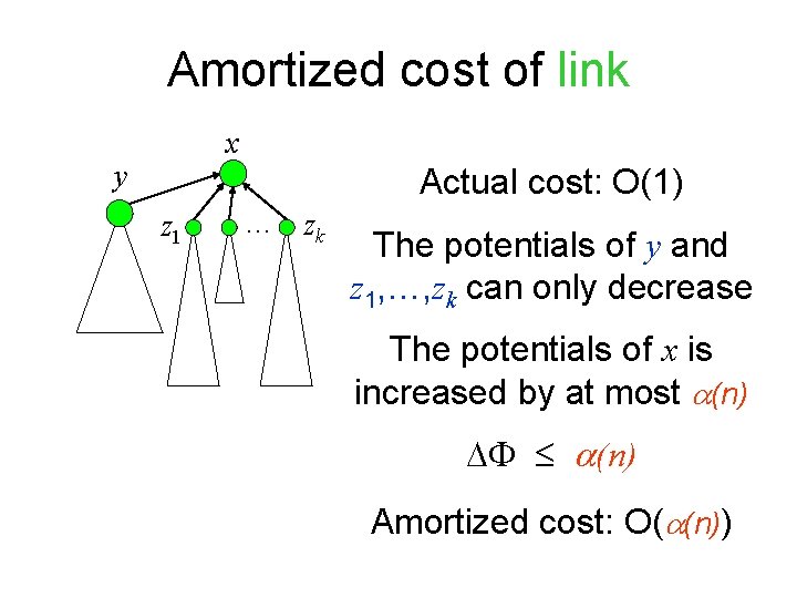
Amortized cost of link x y Actual cost: O(1) z 1 … zk The potentials of y and z 1, …, zk can only decrease The potentials of x is increased by at most (n) Amortized cost: O( (n))

Amortized cost of find y=p’[x] rank[x] is unchanged rank[p[x]] is increased level(x) is either unchanged or is increased p[x] x If level(x) is unchanged, then index(x) is either unchanged or is increased If level(x) is increased, then index(x) is decreased by at most rank[x]– 1 is either unchanged or is decreased

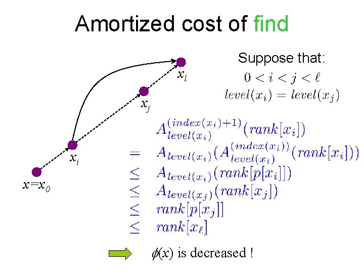
Amortized cost of find xl Suppose that: xj xi x=x 0 (x) is decreased !

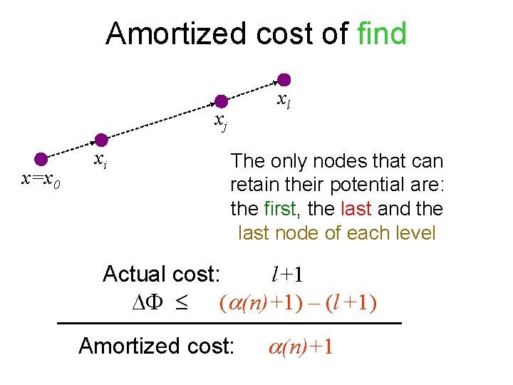
Amortized cost of find xj x=x 0 xi xl The only nodes that can retain their potential are: the first, the last and the last node of each level Actual cost: l +1 ( (n)+1) – (l +1) Amortized cost: (n)+1