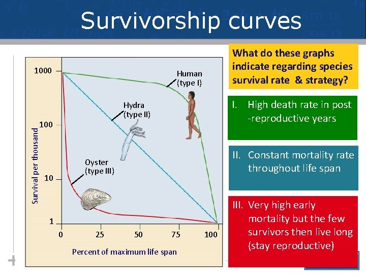
Survivorship curves 1000 Human type I I High

Survivorship curves 1000 Human (type I) I. High death rate in post -reproductive years Hydra (type II) 100 Survival per thousand What do these graphs indicate regarding species survival rate & strategy? II. Constant mortality rate throughout life span Oyster (type III) 10 1 0 25 50 75 Percent of maximum life span 100 III. Very high early mortality but the few survivors then live long (stay reproductive)

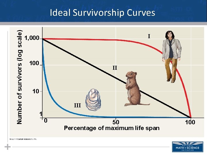
Number of survivors (log scale) Ideal Survivorship Curves I 1, 000 100 II 10 III 1 0 50 Percentage of maximum life span 100

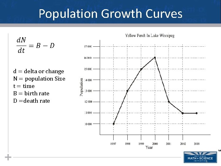
Population Growth Curves d = delta or change N = population Size t = time B = birth rate D =death rate 4

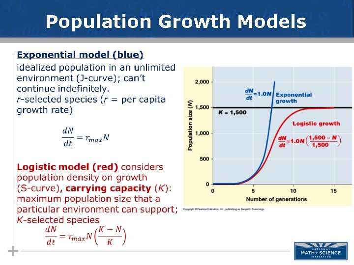
Population Growth Models •

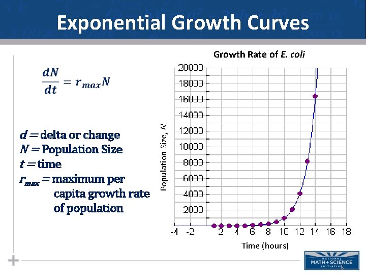
Exponential Growth Curves Growth Rate of E. coli d = delta or change N = Population Size t = time rmax = maximum per capita growth rate of population Population Size, N Time (hours) 6

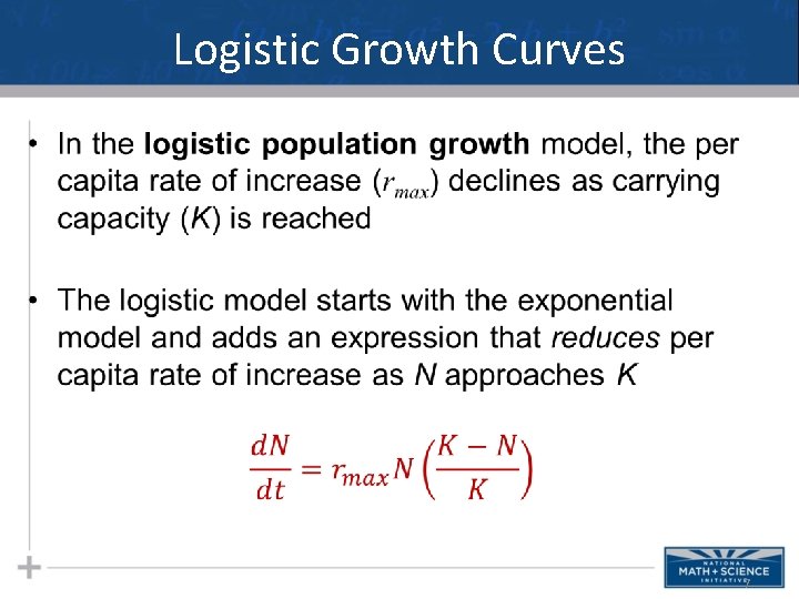
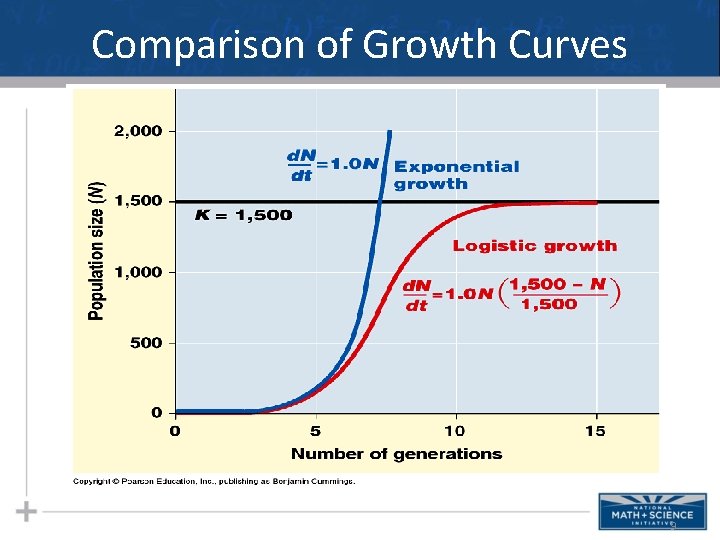
Logistic Growth Curves 7

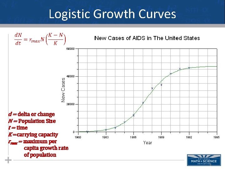
Logistic Growth Curves d = delta or change N = Population Size t = time K =carrying capacity rmax = maximum per capita growth rate of population 8

Comparison of Growth Curves 9

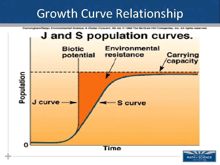
Growth Curve Relationship 10

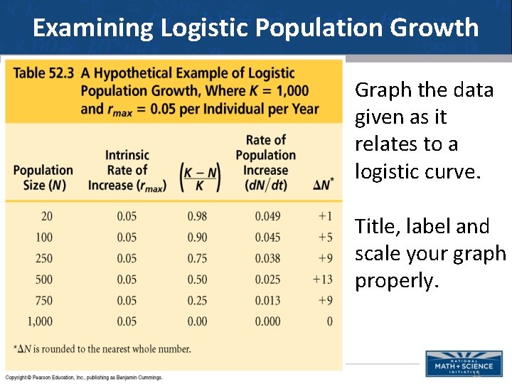
Examining Logistic Population Growth Graph the data given as it relates to a logistic curve. Title, label and scale your graph properly. 11

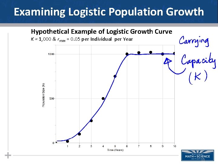
Examining Logistic Population Growth Hypothetical Example of Logistic Growth Curve K = 1, 000 & rmax = 0. 05 per Individual per Year 12

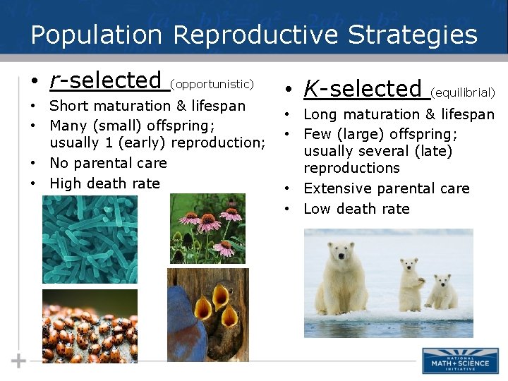
Population Reproductive Strategies • r-selected (opportunistic) • Short maturation & lifespan • Many (small) offspring; usually 1 (early) reproduction; • No parental care • High death rate • K-selected (equilibrial) • Long maturation & lifespan • Few (large) offspring; usually several (late) reproductions • Extensive parental care • Low death rate

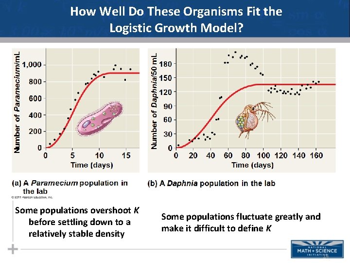
How Well Do These Organisms Fit the Logistic Growth Model? Some populations overshoot K before settling down to a relatively stable density Some populations fluctuate greatly and make it difficult to define K 14

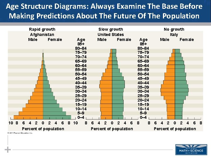
Age Structure Diagrams: Always Examine The Base Before Making Predictions About The Future Of The Population Rapid growth Afghanistan Male Female 10 8 6 4 2 0 2 4 6 Percent of population Age 85+ 80– 84 75– 79 70– 74 65– 69 60– 64 55– 59 50– 54 45– 49 40– 44 35– 39 30– 34 25– 29 20– 24 15– 19 10– 14 5– 9 0– 4 8 10 8 Slow growth United States Male Female 6 4 2 0 2 4 6 Percent of population Age 85+ 80– 84 75– 79 70– 74 65– 69 60– 64 55– 59 50– 54 45– 49 40– 44 35– 39 30– 34 25– 29 20– 24 15– 19 10– 14 5– 9 0– 4 8 8 No growth Italy Male Female 6 4 2 0 2 4 6 8 Percent of population

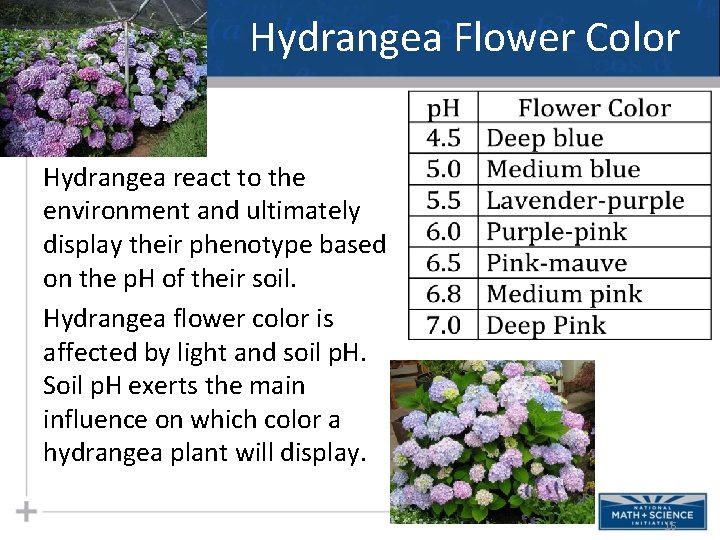
Hydrangea Flower Color Hydrangea react to the environment and ultimately display their phenotype based on the p. H of their soil. Hydrangea flower color is affected by light and soil p. H. Soil p. H exerts the main influence on which color a hydrangea plant will display. 16

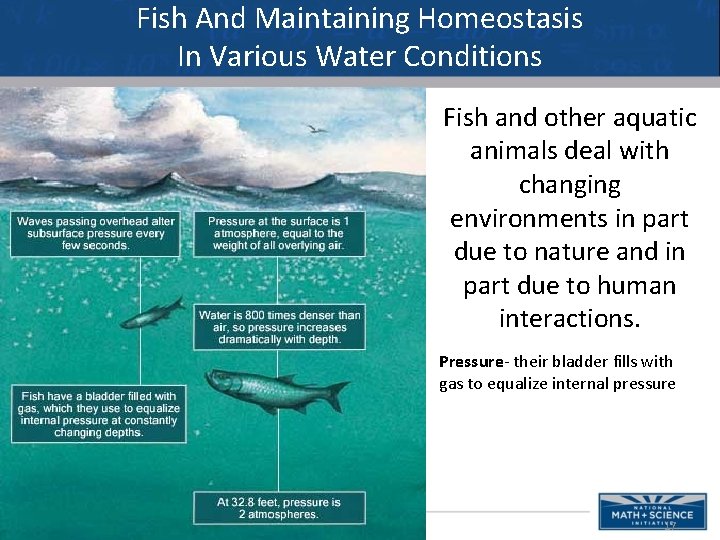
Fish And Maintaining Homeostasis In Various Water Conditions Fish and other aquatic animals deal with changing environments in part due to nature and in part due to human interactions. Pressure- their bladder fills with gas to equalize internal pressure 17

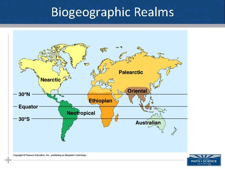
Biogeographic Realms 18

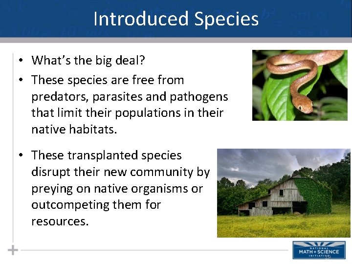
Introduced Species • What’s the big deal? • These species are free from predators, parasites and pathogens that limit their populations in their native habitats. • These transplanted species disrupt their new community by preying on native organisms or outcompeting them for resources. 19

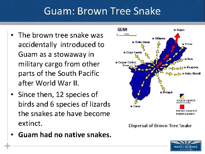
Guam: Brown Tree Snake • The brown tree snake was accidentally introduced to Guam as a stowaway in military cargo from other parts of the South Pacific after World War II. • Since then, 12 species of birds and 6 species of lizards the snakes ate have become extinct. • Guam had no native snakes. Dispersal of Brown Tree Snake 20

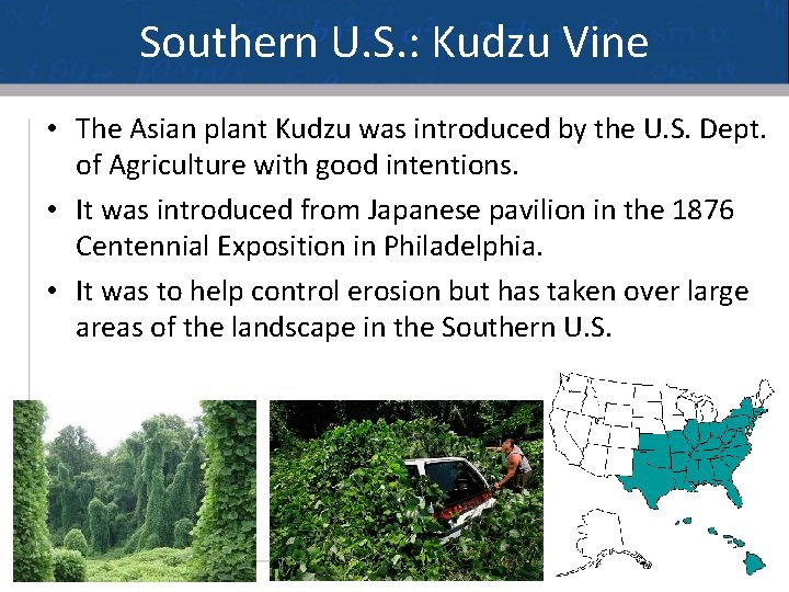
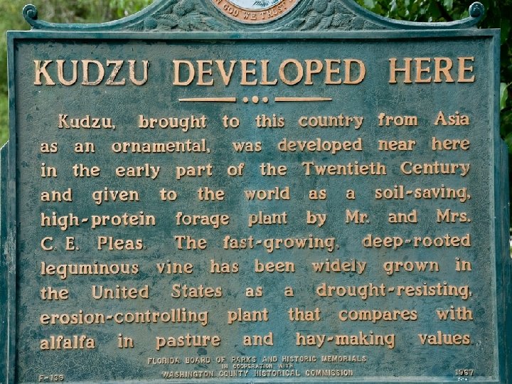
Southern U. S. : Kudzu Vine • The Asian plant Kudzu was introduced by the U. S. Dept. of Agriculture with good intentions. • It was introduced from Japanese pavilion in the 1876 Centennial Exposition in Philadelphia. • It was to help control erosion but has taken over large areas of the landscape in the Southern U. S. 21

Introduced Species 22

New York: European Starling • From the New York Times, 1990 The year was 1890 when an eccentric drug manufacturer named Eugene Schieffelin entered New York City's Central Park and released some 60 European starlings he had imported from England. In 1891 he loosed 40 more. Schieffelin's motives were as romantic as they were ill fated: he hoped to introduce into North America every bird mentioned by Shakespeare. Skylarks and song thrushes failed to thrive, but the enormity of his success with starlings continues to haunt us. This centennial year is worth observing as an object lesson in how even noble intentions can lead to disaster when humanity meddles with nature. 23

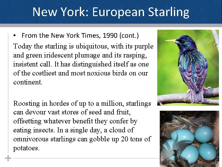
New York: European Starling • From the New York Times, 1990 (cont. ) Today the starling is ubiquitous, with its purple and green iridescent plumage and its rasping, insistent call. It has distinguished itself as one of the costliest and most noxious birds on our continent. Roosting in hordes of up to a million, starlings can devour vast stores of seed and fruit, offsetting whatever benefit they confer by eating insects. In a single day, a cloud of omnivorous starlings can gobble up 20 tons of potatoes. 24

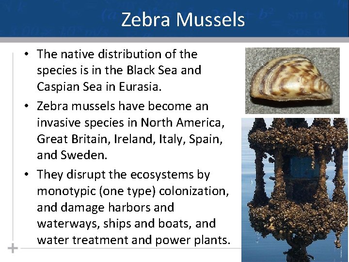
Zebra Mussels • The native distribution of the species is in the Black Sea and Caspian Sea in Eurasia. • Zebra mussels have become an invasive species in North America, Great Britain, Ireland, Italy, Spain, and Sweden. • They disrupt the ecosystems by monotypic (one type) colonization, and damage harbors and waterways, ships and boats, and water treatment and power plants. 25

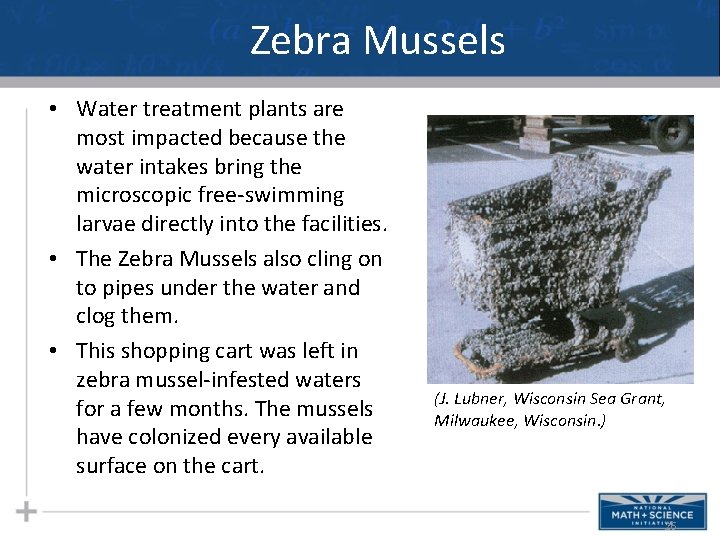
Zebra Mussels • Water treatment plants are most impacted because the water intakes bring the microscopic free-swimming larvae directly into the facilities. • The Zebra Mussels also cling on to pipes under the water and clog them. • This shopping cart was left in zebra mussel-infested waters for a few months. The mussels have colonized every available surface on the cart. (J. Lubner, Wisconsin Sea Grant, Milwaukee, Wisconsin. ) 26

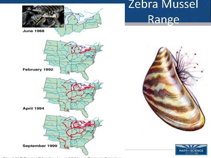
Zebra Mussel Range 27

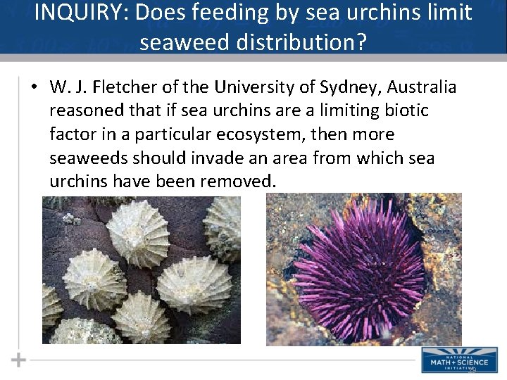
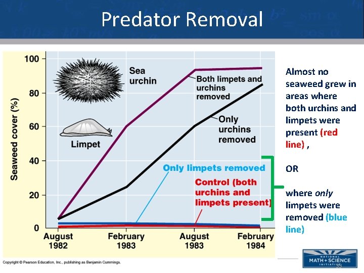
INQUIRY: Does feeding by sea urchins limit seaweed distribution? • W. J. Fletcher of the University of Sydney, Australia reasoned that if sea urchins are a limiting biotic factor in a particular ecosystem, then more seaweeds should invade an area from which sea urchins have been removed. 29

INQUIRY: Does feeding by sea urchins limit seaweed distribution? • Seems reasonable and a tad obvious, but the area is also occupied by seaweed-eating mollusc called limpets. • What to do? Formulate an experimental design aimed at answering the inquiry question. 30

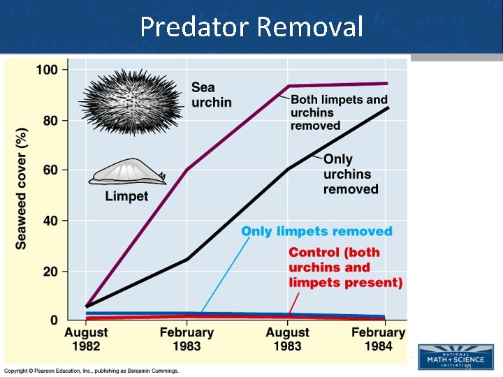
Predator Removal 31

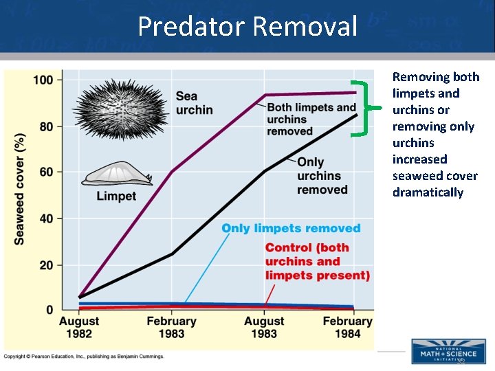
Predator Removal Removing both limpets and urchins or removing only urchins increased seaweed cover dramatically 32

Predator Removal Almost no seaweed grew in areas where both urchins and limpets were present (red line) , OR where only limpets were removed (blue line) 33

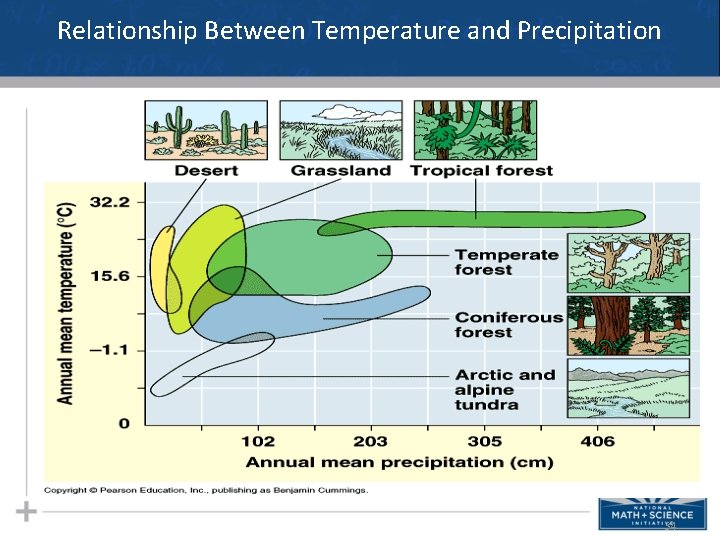
Relationship Between Temperature and Precipitation 34

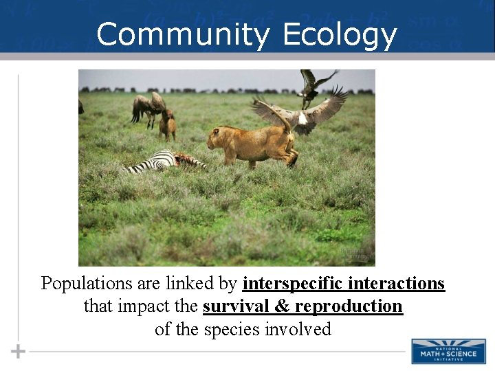
Community Ecology Populations are linked by interspecific interactions that impact the survival & reproduction of the species involved

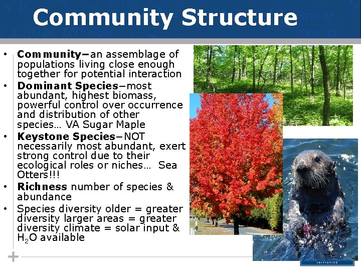
Community Structure • Community−an assemblage of populations living close enough together for potential interaction • Dominant Species−most abundant, highest biomass, powerful control over occurrence and distribution of other species… VA Sugar Maple • Keystone Species−NOT necessarily most abundant, exert strong control due to their ecological roles or niches… Sea Otters!!! • Richness number of species & abundance • Species diversity older = greater diversity larger areas = greater diversity climate = solar input & H 2 O available

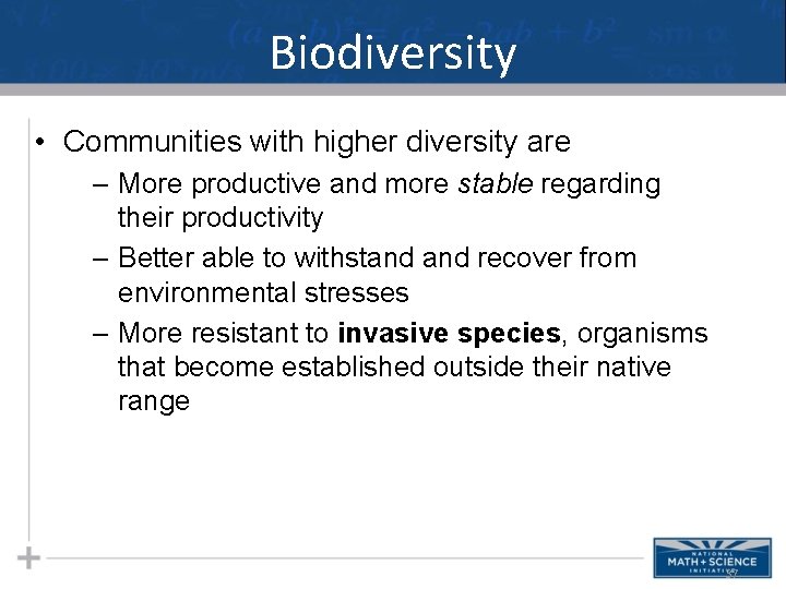
Biodiversity • Communities with higher diversity are – More productive and more stable regarding their productivity – Better able to withstand recover from environmental stresses – More resistant to invasive species, organisms that become established outside their native range 37

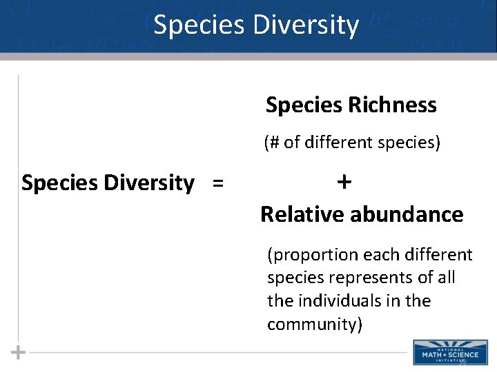
Species Diversity Species Richness (# of different species) Species Diversity = + Relative abundance (proportion each different species represents of all the individuals in the community) 38

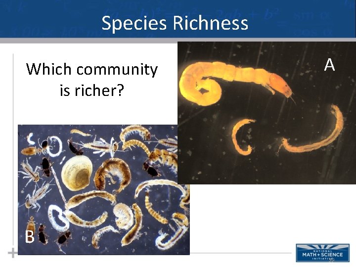
Species Richness Which community is richer? A B 39

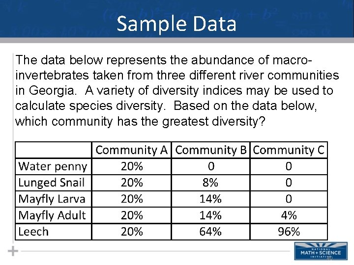
Sample Data The data below represents the abundance of macroinvertebrates taken from three different river communities in Georgia. A variety of diversity indices may be used to calculate species diversity. Based on the data below, which community has the greatest diversity? 40

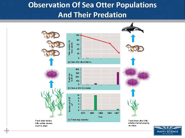
Observation Of Sea Otter Populations And Their Predation Otter number (% max. count) 100 80 60 40 20 0 (a) Sea otter abundance Grams per 0. 25 m 2 400 300 200 100 0 Number per 0. 25 m 2 (b) Sea urchin biomass 10 8 6 4 2 0 1972 1985 1989 1993 1997 Year Food chain before killer whale involvement in chain (c) Total kelp density Food chain after killer whales started preying on otters

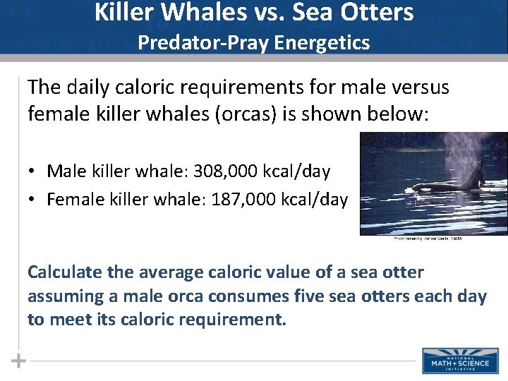
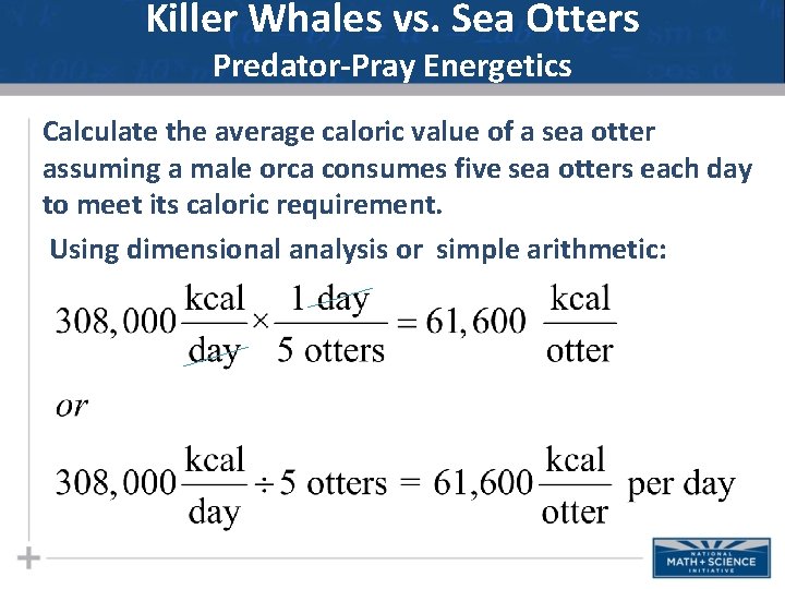
Killer Whales vs. Sea Otters Predator-Pray Energetics The daily caloric requirements for male versus female killer whales (orcas) is shown below: • Male killer whale: 308, 000 kcal/day • Female killer whale: 187, 000 kcal/day Calculate the average caloric value of a sea otter assuming a male orca consumes five sea otters each day to meet its caloric requirement.

Killer Whales vs. Sea Otters Predator-Pray Energetics Calculate the average caloric value of a sea otter assuming a male orca consumes five sea otters each day to meet its caloric requirement. Using dimensional analysis or simple arithmetic:

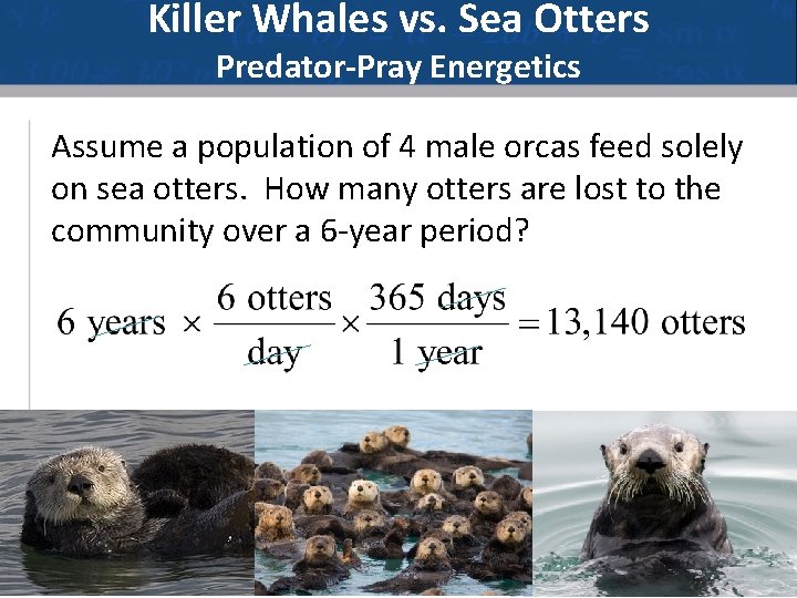
Killer Whales vs. Sea Otters Predator-Pray Energetics Assume a population of 4 male orcas feed solely on sea otters. How many otters are lost to the community over a 6 -year period?

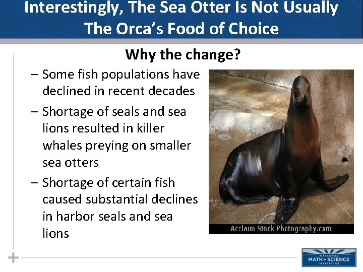
Interestingly, The Sea Otter Is Not Usually The Orca’s Food of Choice Why the change? – Some fish populations have declined in recent decades – Shortage of seals and sea lions resulted in killer whales preying on smaller sea otters – Shortage of certain fish caused substantial declines in harbor seals and sea lions

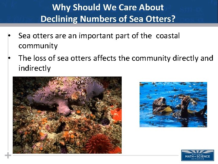
Why Should We Care About Declining Numbers of Sea Otters? • Sea otters are an important part of the coastal community • The loss of sea otters affects the community directly and indirectly

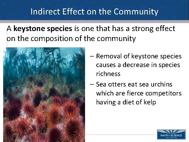
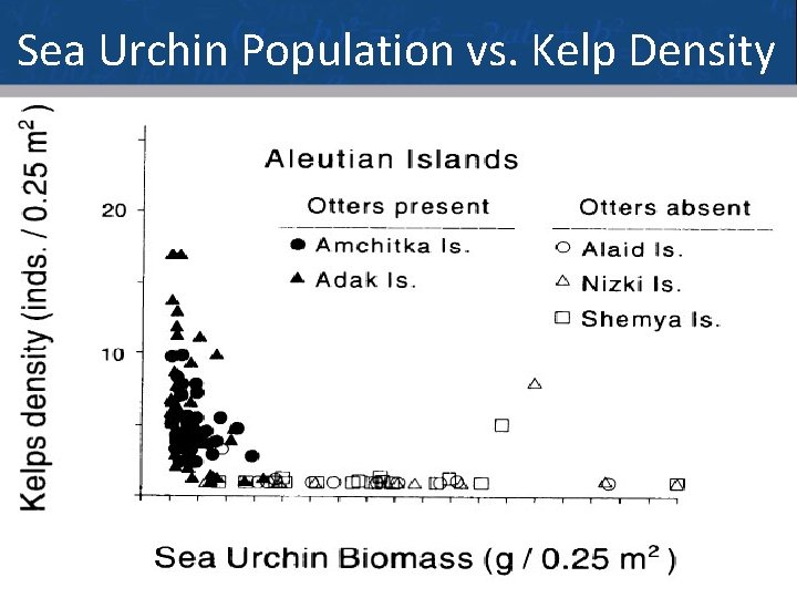
Indirect Effect on the Community A keystone species is one that has a strong effect on the composition of the community – Removal of keystone species causes a decrease in species richness – Sea otters eat sea urchins which are fierce competitors having a diet of kelp

Sea Urchin Population vs. Kelp Density 48

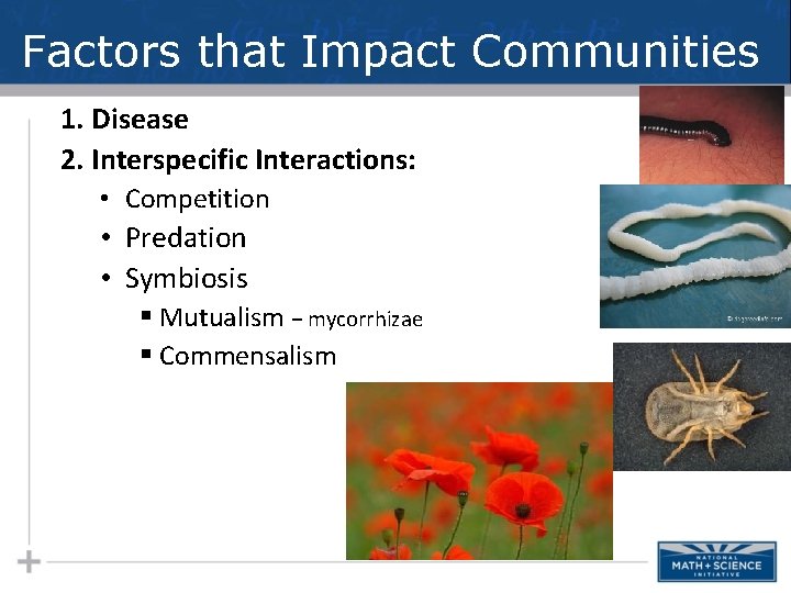
Factors that Impact Communities 1. Disease 2. Interspecific Interactions: • Competition • Predation • Symbiosis § Mutualism − mycorrhizae § Commensalism

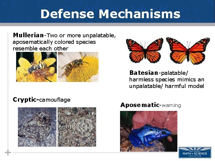
Defense Mechanisms Mullerian-Two or more unpalatable, aposematically colored species resemble each other Batesian-palatable/ harmless species mimics an unpalatable/ harmful model Cryptic-camouflage Aposematic-warning

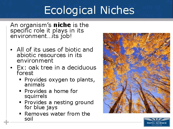
Ecological Niches An organism’s niche is the specific role it plays in its environment…its job! • All of its uses of biotic and abiotic resources in its environment • Ex: oak tree in a deciduous forest § Provides oxygen to plants, animals § Provides a home for squirrels § Provides a nesting ground for blue jays § Removes water from the soil

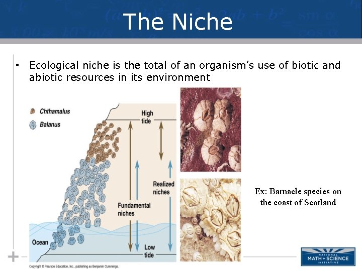
The Niche • Ecological niche is the total of an organism’s use of biotic and abiotic resources in its environment Ex: Barnacle species on the coast of Scotland

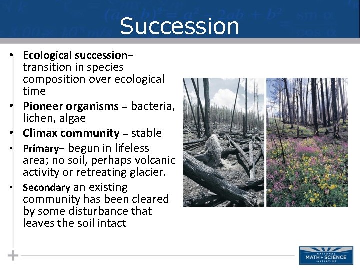
Succession • Ecological succession− transition in species composition over ecological time • Pioneer organisms = bacteria, lichen, algae • Climax community = stable • Primary− begun in lifeless area; no soil, perhaps volcanic activity or retreating glacier. • Secondary an existing community has been cleared by some disturbance that leaves the soil intact

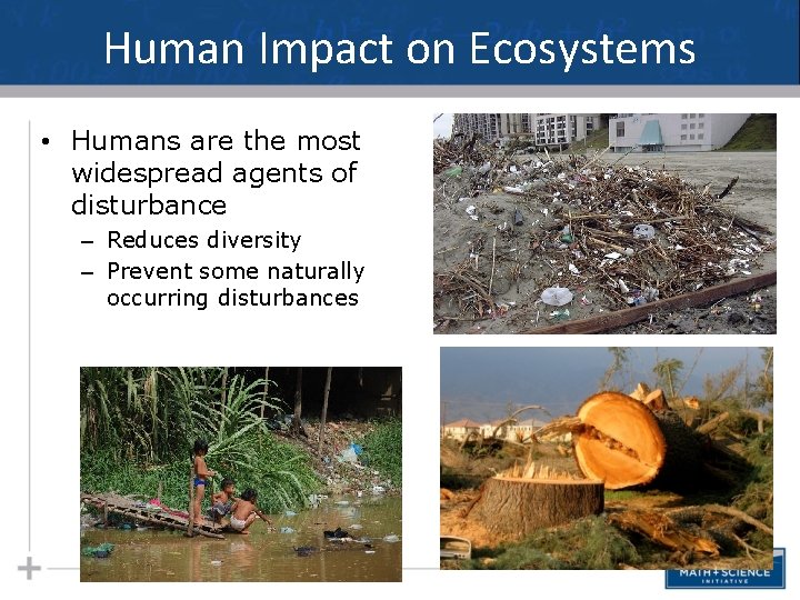
Human Impact on Ecosystems • Humans are the most widespread agents of disturbance – Reduces diversity – Prevent some naturally occurring disturbances

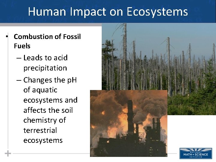
Human Impact on Ecosystems • Combustion of Fossil Fuels – Leads to acid precipitation – Changes the p. H of aquatic ecosystems and affects the soil chemistry of terrestrial ecosystems

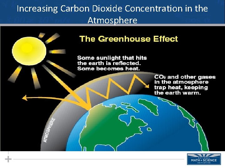
Increasing Carbon Dioxide Concentration in the Atmosphere

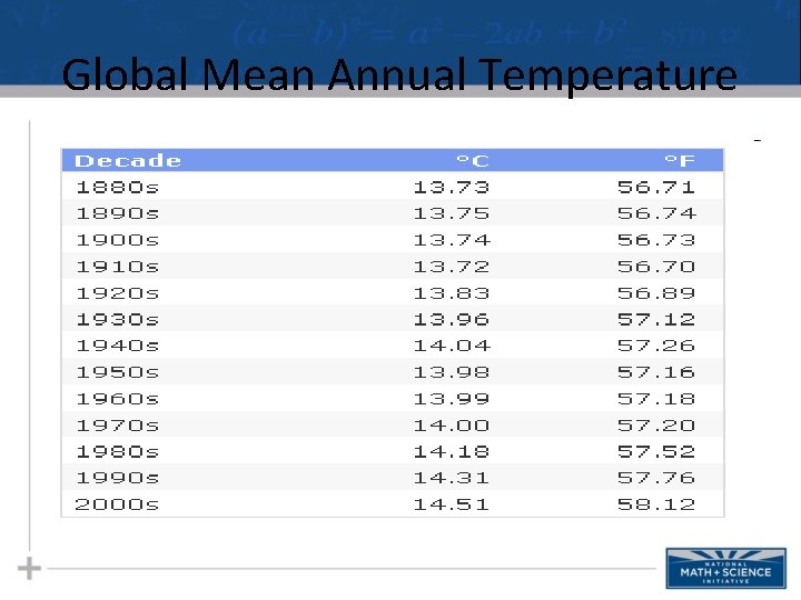
Global Mean Annual Temperature

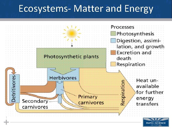
Ecosystems- Matter and Energy 58

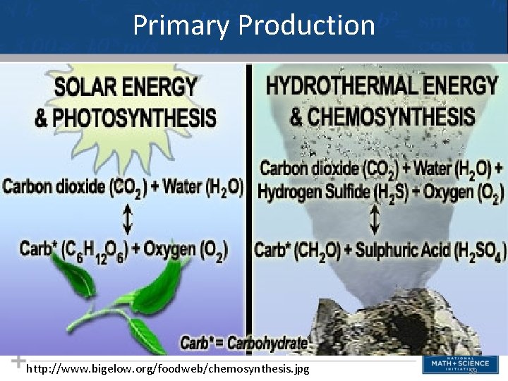
Primary Production http: //www. bigelow. org/foodweb/chemosynthesis. jpg 59

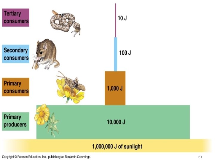
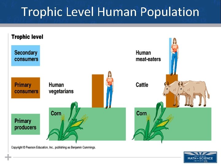
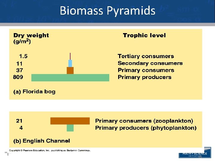
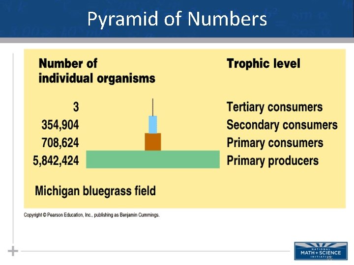
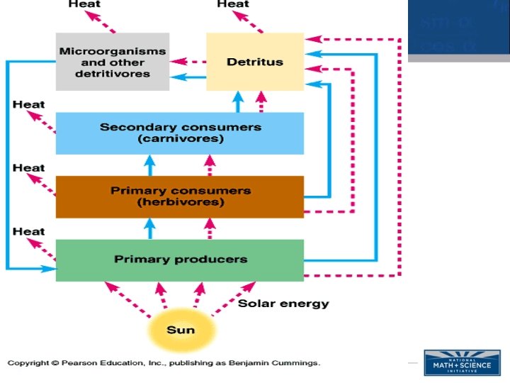
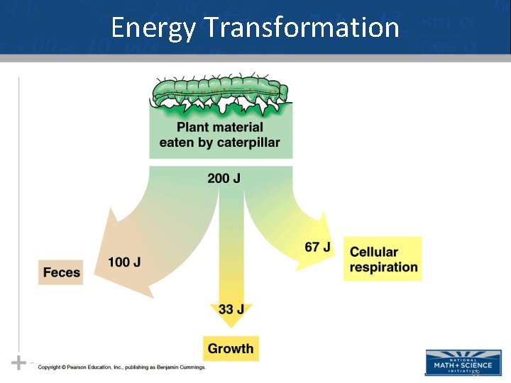
Visualizing Matter & Energy There a variety of diagrams that help us visualize how energy, biomass, matter, and even number of organisms interact in a particular community or ecosystem. It is important that you look carefully at the diagrams and understand what it says about that ecosystem in terms of matter and/or energy. 60

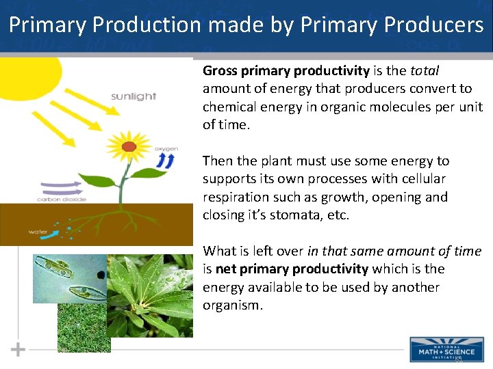
Primary Production made by Primary Producers Gross primary productivity is the total amount of energy that producers convert to chemical energy in organic molecules per unit of time. Then the plant must use some energy to supports its own processes with cellular respiration such as growth, opening and closing it’s stomata, etc. What is left over in that same amount of time is net primary productivity which is the energy available to be used by another organism. 61

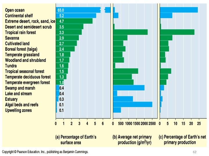
Primary Production 62

Net Product Pyramid 63

Trophic Level Human Population 64

Biomass Pyramids • I think this slide should go up with the other pyramid slides even though it’s about populations 65

Pyramid of Numbers 66

Energy Transformation 68

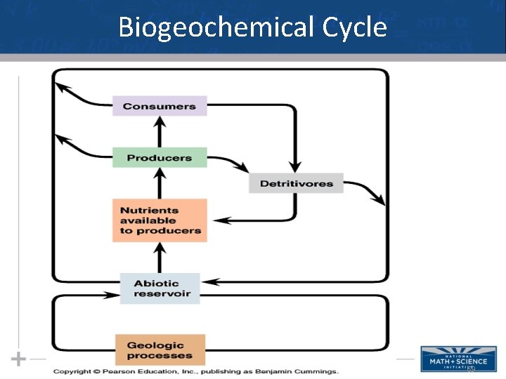
Biogeochemical Cycle 69

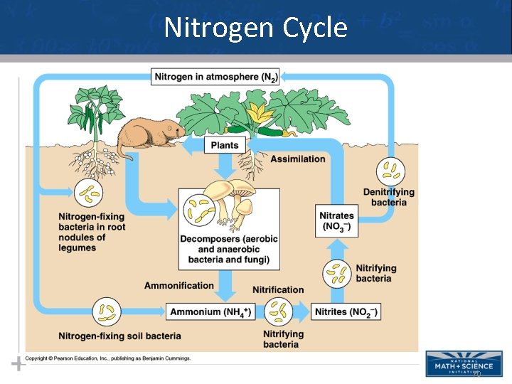
Nitrogen Cycle 70

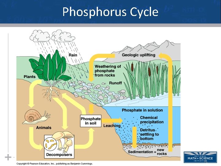
Phosphorus Cycle 71

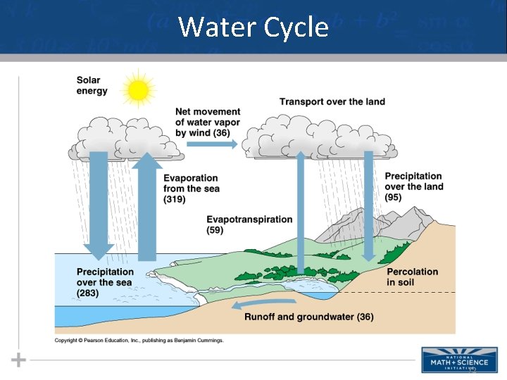
Water Cycle 72

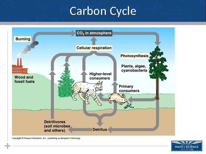
Carbon Cycle 73

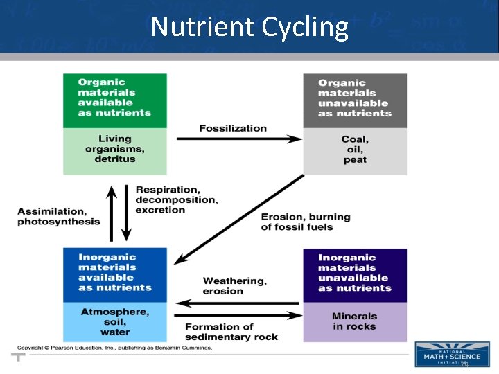
Nutrient Cycling 74

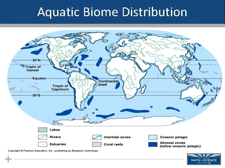
Aquatic Biome Distribution 75

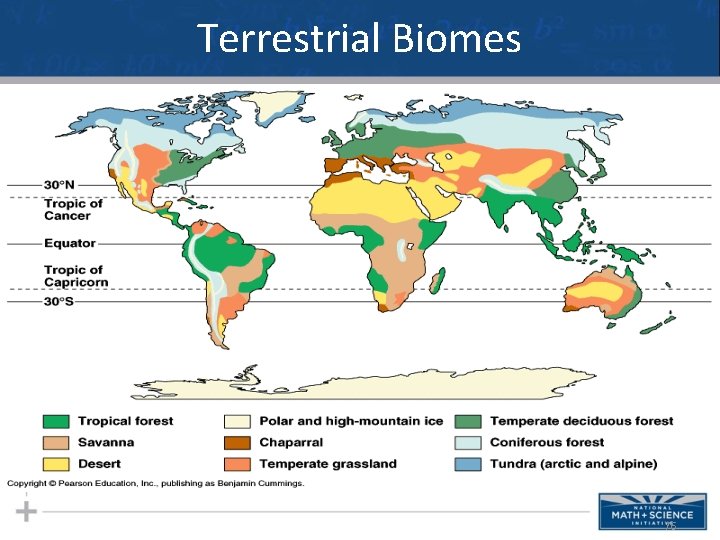
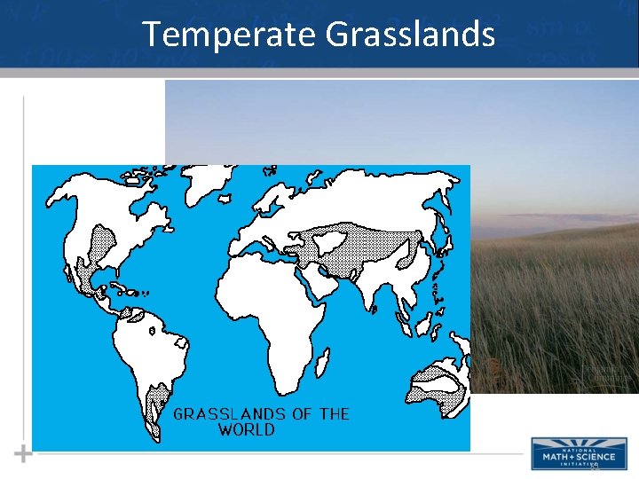
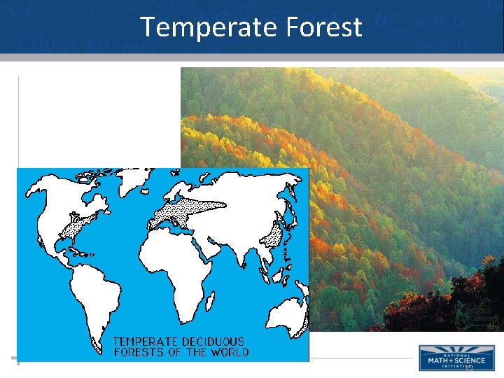
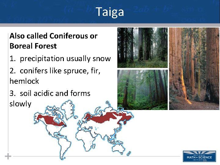
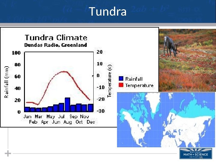
Terrestrial Biomes 76

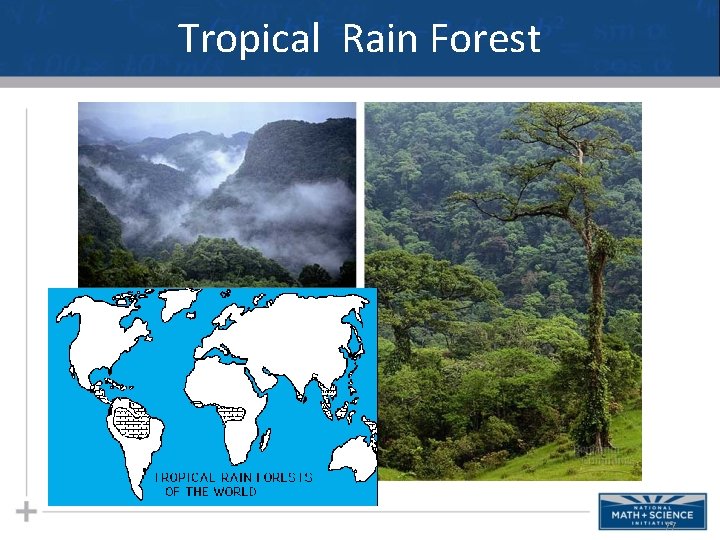
Tropical Rain Forest 77

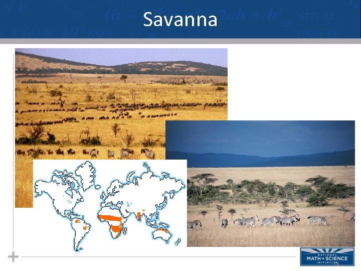
Savanna 78

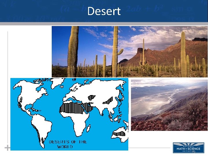
Desert 79

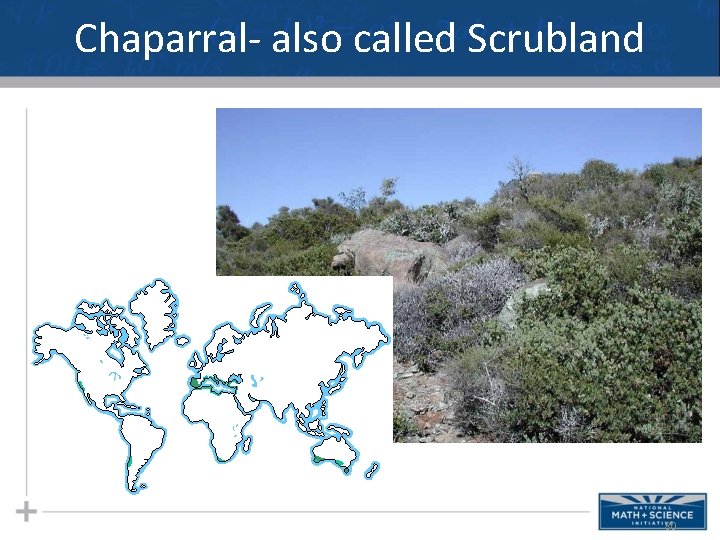
Chaparral- also called Scrubland 80

Temperate Grasslands 81

Temperate Forest 82

Taiga Also called Coniferous or Boreal Forest 1. precipitation usually snow 2. conifers like spruce, fir, hemlock 3. soil acidic and forms slowly 83

Tundra 84

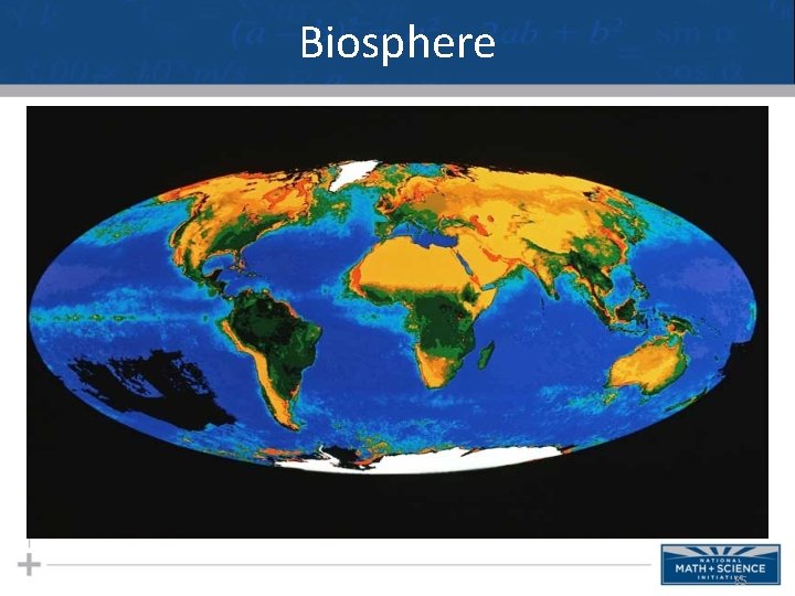
Biosphere 85

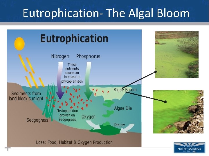
Eutrophication- The Algal Bloom 86