Session 11 Introduction to Options Option Properties Option

Session 11: Introduction to Options: Option Properties, Option Payoffs This session begins the second portion of the course, which focuses on options. The development of option theory is one of the major triumphs of modern finance. It has contributed to enormous growth and proliferation of trading in derivative securities, as well as the use of new theoretical valuation tools for derivatives valuation and risk management In 1997 the Nobel Prize was awarded to Myron Scholes and Robert Merton in recognition of the importance of the option pricing model. Fischer Black would surely have shared the award, but he unfortunately died in 1995, before it was given. Session 11 describes the basic properties of calls and puts and the markets for them. It also illustrates the payoffs on several standard option positions. FINC-UB. 0043 Futures and Options Spring 2017 Part II: Option Pricing and Hedging © 2017 Figlewski 1

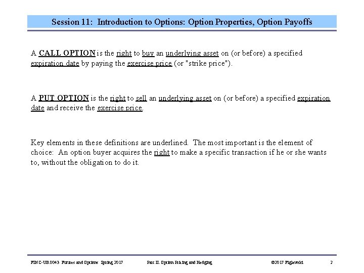
Session 11: Introduction to Options: Option Properties, Option Payoffs A CALL OPTION is the right to buy an underlying asset on (or before) a specified expiration date by paying the exercise price (or "strike price"). A PUT OPTION is the right to sell an underlying asset on (or before) a specified expiration date and receive the exercise price. Key elements in these definitions are underlined. The most important is the element of choice: An option buyer acquires the right to make a specific transaction if he or she wants to, without the obligation to do it. FINC-UB. 0043 Futures and Options Spring 2017 Part II: Option Pricing and Hedging © 2017 Figlewski 2

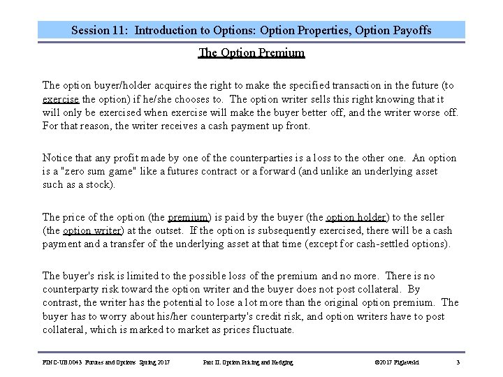
Session 11: Introduction to Options: Option Properties, Option Payoffs The Option Premium The option buyer/holder acquires the right to make the specified transaction in the future (to exercise the option) if he/she chooses to. The option writer sells this right knowing that it will only be exercised when exercise will make the buyer better off, and the writer worse off. For that reason, the writer receives a cash payment up front. Notice that any profit made by one of the counterparties is a loss to the other one. An option is a "zero sum game" like a futures contract or a forward (and unlike an underlying asset such as a stock). The price of the option (the premium) is paid by the buyer (the option holder) to the seller (the option writer) at the outset. If the option is subsequently exercised, there will be a cash payment and a transfer of the underlying asset at that time (except for cash-settled options). The buyer's risk is limited to the possible loss of the premium and no more. There is no counterparty risk toward the option writer and the buyer does not post collateral. By contrast, the writer has the potential to lose a lot more than the original option premium. The buyer has to worry about his/her counterparty's credit risk, and option writers have to post collateral, which is marked to market as prices fluctuate. FINC-UB. 0043 Futures and Options Spring 2017 Part II: Option Pricing and Hedging © 2017 Figlewski 3

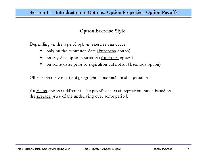
Session 11: Introduction to Options: Option Properties, Option Payoffs Option Exercise Style Depending on the type of option, exercise can occur • only on the expiration date (European option) • on any date up to expiration (American option) • on some dates prior to expiration but not all (Bermuda option) Other exercise terms (and geographical names) are also possible. An Asian option is different: The payoff occurs at expiration, but is based on the average price of the underlying over some period. FINC-UB. 0043 Futures and Options Spring 2017 Part II: Option Pricing and Hedging © 2017 Figlewski 4

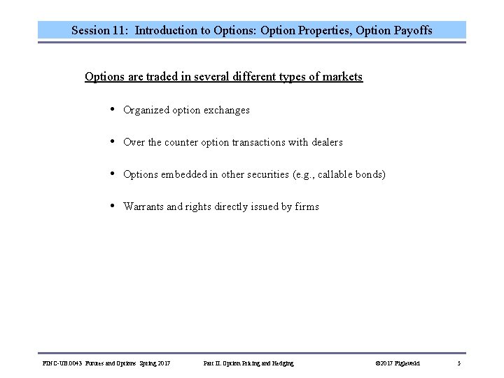
Session 11: Introduction to Options: Option Properties, Option Payoffs Options are traded in several different types of markets • Organized option exchanges • Over the counter option transactions with dealers • Options embedded in other securities (e. g. , callable bonds) • Warrants and rights directly issued by firms FINC-UB. 0043 Futures and Options Spring 2017 Part II: Option Pricing and Hedging © 2017 Figlewski 5

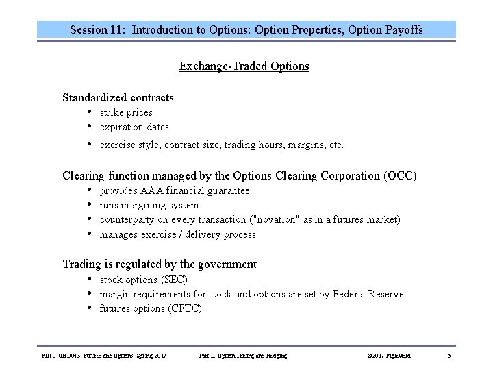
Session 11: Introduction to Options: Option Properties, Option Payoffs Exchange-Traded Options Standardized contracts • • • strike prices expiration dates exercise style, contract size, trading hours, margins, etc. Clearing function managed by the Options Clearing Corporation (OCC) • • provides AAA financial guarantee runs margining system counterparty on every transaction ("novation" as in a futures market) manages exercise / delivery process Trading is regulated by the government • • • stock options (SEC) margin requirements for stock and options are set by Federal Reserve futures options (CFTC) FINC-UB. 0043 Futures and Options Spring 2017 Part II: Option Pricing and Hedging © 2017 Figlewski 6

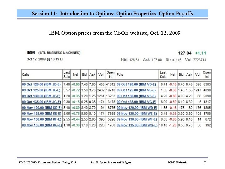
Session 11: Introduction to Options: Option Properties, Option Payoffs IBM Option prices from the CBOE website, Oct. 12, 2009 FINC-UB. 0043 Futures and Options Spring 2017 Part II: Option Pricing and Hedging © 2017 Figlewski 7

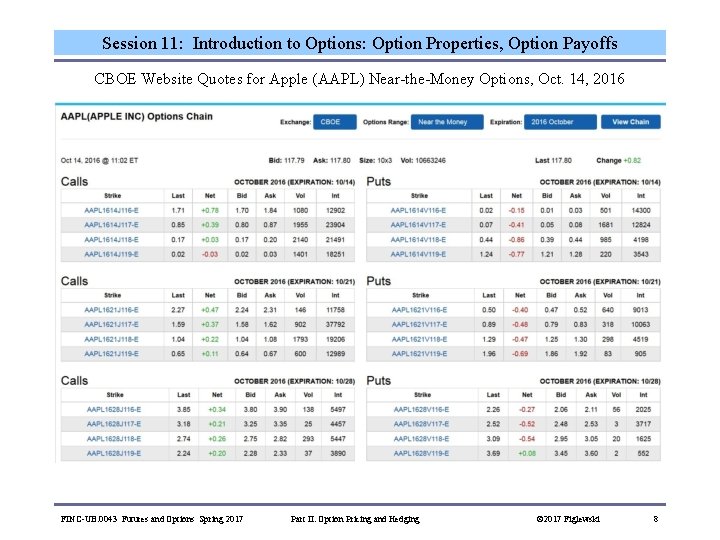
Session 11: Introduction to Options: Option Properties, Option Payoffs CBOE Website Quotes for Apple (AAPL) Near-the-Money Options, Oct. 14, 2016 FINC-UB. 0043 Futures and Options Spring 2017 Part II: Option Pricing and Hedging © 2017 Figlewski 8

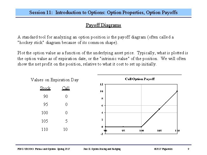
Session 11: Introduction to Options: Option Properties, Option Payoffs Payoff Diagrams A standard tool for analyzing an option position is the payoff diagram (often called a "hockey stick" diagram because of its common shape). Plot the option value as a function of the underlying asset price. Typically, what is plotted is the option value as of expiration date, or the "intrinsic value" of the position. We will often show the net profit on the position, relative to what it cost to set up initially. Values on Expiration Day Stock Call 90 95 0 100 0 105 5 110 10 FINC-UB. 0043 Futures and Options Spring 2017 Part II: Option Pricing and Hedging © 2017 Figlewski 9

Session 11: Introduction to Options: Option Properties, Option Payoffs Here's What a Hockey Stick Looks Like (in case you didn't know): FINC-UB. 0043 Futures and Options Spring 2017 Part II: Option Pricing and Hedging © 2017 Figlewski 10

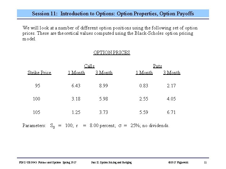
Session 11: Introduction to Options: Option Properties, Option Payoffs We will look at a number of different option positions using the following set of option prices. These are theoretical values computed using the Black-Scholes option pricing model. OPTION PRICES Strike Price 95 100 105 Calls 1 Month 3 Month Puts 1 Month 3 Month 6. 43 8. 99 0. 83 2. 17 3. 18 5. 98 2. 55 4. 05 1. 25 3. 73 5. 59 6. 71 Parameters: S 0 = 100; r = 8. 00 percent; = 25%; no dividends. FINC-UB. 0043 Futures and Options Spring 2017 Part II: Option Pricing and Hedging © 2017 Figlewski 11

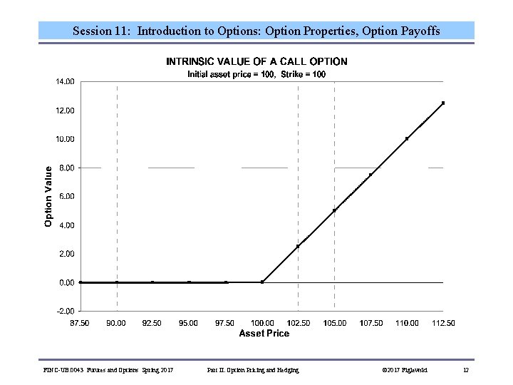
Session 11: Introduction to Options: Option Properties, Option Payoffs FINC-UB. 0043 Futures and Options Spring 2017 Part II: Option Pricing and Hedging © 2017 Figlewski 12

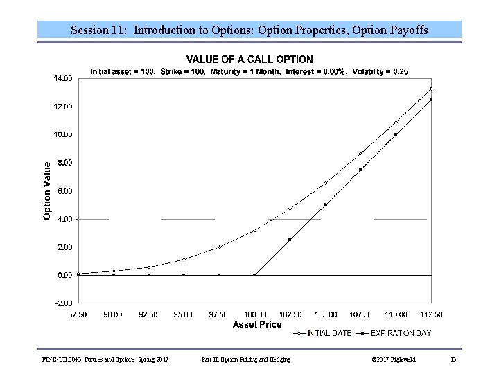
Session 11: Introduction to Options: Option Properties, Option Payoffs FINC-UB. 0043 Futures and Options Spring 2017 Part II: Option Pricing and Hedging © 2017 Figlewski 13

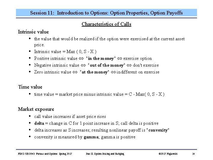
Session 11: Introduction to Options: Option Properties, Option Payoffs Characteristics of Calls Intrinsic value • • • the value that would be realized if the option were exercised at the current asset price. Intrinsic value = Max ( 0, S - X ) Positive intrinsic value "in the money" exercise option Negative intrinsic value "out of the money" don't exercise Zero intrinsic value "at the money" indifferent on exercise Time value • time value = market price minus intrinsic value = C - Max( 0, S - X ) Market exposure • • call value increases if asset price rises delta = change in C for 1 point increase in S; call delta is positive delta increases as S increases; resulting nonlinear payoff is "convexity" convexity is measured by gamma; gamma is positive FINC-UB. 0043 Futures and Options Spring 2017 Part II: Option Pricing and Hedging © 2017 Figlewski 14

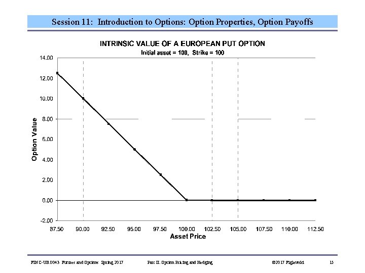
Session 11: Introduction to Options: Option Properties, Option Payoffs FINC-UB. 0043 Futures and Options Spring 2017 Part II: Option Pricing and Hedging © 2017 Figlewski 15

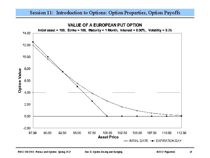
Session 11: Introduction to Options: Option Properties, Option Payoffs FINC-UB. 0043 Futures and Options Spring 2017 Part II: Option Pricing and Hedging © 2017 Figlewski 16

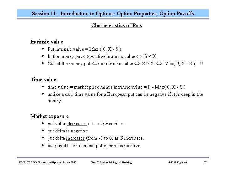
Session 11: Introduction to Options: Option Properties, Option Payoffs Characteristics of Puts Intrinsic value • • • Put intrinsic value = Max ( 0, X - S ) In the money put positive intrinsic value S < X Out of the money put no intrinsic value S > X Max( 0, X - S ) = 0 Time value • • time value = market price minus intrinsic value = P - Max( 0, X - S ) unlike a call, time value for a European put can be negative if it is deep in the money Market exposure • • put value decreases if asset price rises put delta is negative put delta increases (from -1 to 0) as S increases; put payoffs are convex; put gamma is positive FINC-UB. 0043 Futures and Options Spring 2017 Part II: Option Pricing and Hedging © 2017 Figlewski 17

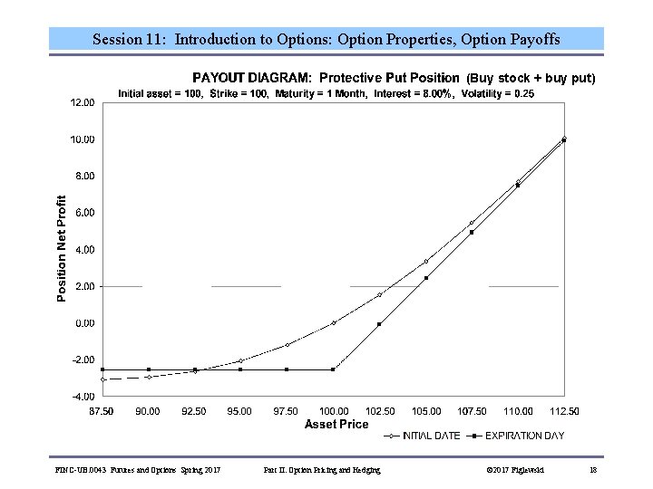
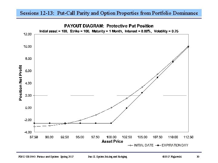
Session 11: Introduction to Options: Option Properties, Option Payoffs (Buy stock + buy put) FINC-UB. 0043 Futures and Options Spring 2017 Part II: Option Pricing and Hedging © 2017 Figlewski 18

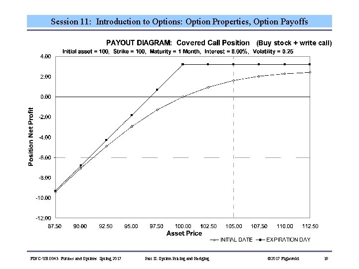
Session 11: Introduction to Options: Option Properties, Option Payoffs (Buy stock + write call) FINC-UB. 0043 Futures and Options Spring 2017 Part II: Option Pricing and Hedging © 2017 Figlewski 19

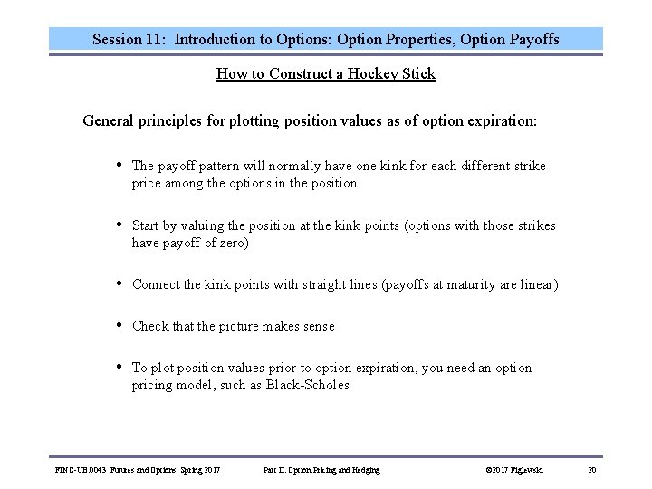
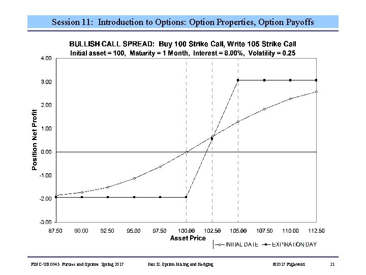
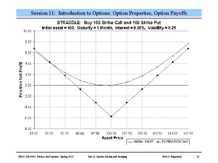
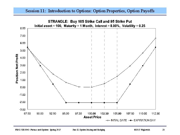
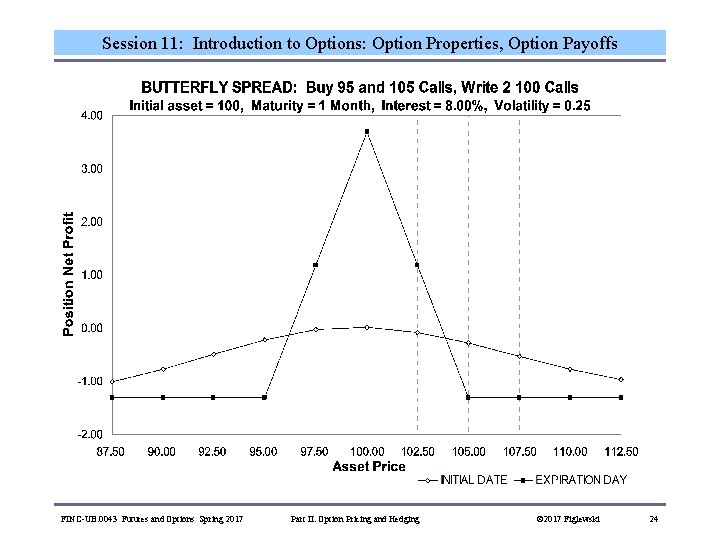
Session 11: Introduction to Options: Option Properties, Option Payoffs How to Construct a Hockey Stick General principles for plotting position values as of option expiration: • The payoff pattern will normally have one kink for each different strike price among the options in the position • Start by valuing the position at the kink points (options with those strikes have payoff of zero) • Connect the kink points with straight lines (payoffs at maturity are linear) • Check that the picture makes sense • To plot position values prior to option expiration, you need an option pricing model, such as Black-Scholes FINC-UB. 0043 Futures and Options Spring 2017 Part II: Option Pricing and Hedging © 2017 Figlewski 20

Session 11: Introduction to Options: Option Properties, Option Payoffs FINC-UB. 0043 Futures and Options Spring 2017 Part II: Option Pricing and Hedging © 2017 Figlewski 21

Session 11: Introduction to Options: Option Properties, Option Payoffs FINC-UB. 0043 Futures and Options Spring 2017 Part II: Option Pricing and Hedging © 2017 Figlewski 22

Session 11: Introduction to Options: Option Properties, Option Payoffs FINC-UB. 0043 Futures and Options Spring 2017 Part II: Option Pricing and Hedging © 2017 Figlewski 23

Session 11: Introduction to Options: Option Properties, Option Payoffs FINC-UB. 0043 Futures and Options Spring 2017 Part II: Option Pricing and Hedging © 2017 Figlewski 24

Session 11: Introduction to Options: Option Properties, Option Payoffs FINC-UB. 0043 Futures and Options Spring 2017 Part II: Option Pricing and Hedging © 2017 Figlewski 25

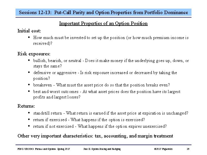
Sessions 12 -13: Put-Call Parity and Option Properties from Portfolio Dominance Important Properties of an Option Position Initial cost: • How much must be invested to set up the position (or how much premium income is received)? Risk exposures: • • bullish, bearish, or neutral - Does it make money if the underlying goes up, down, or stays the same? defensive or aggressive - Is risk exposure increased or decreased by taking the position? breakeven - What must the asset price do so that the position breaks even? best and worst outcomes - At what asset prices does the position have its largest profits and largest losses? Returns: • • • standstill return - What return is earned if the asset price at expiration is unchanged? return if exercised - What happens if the option is exercised? return if not exercised - What happens if the option expires unexercised? Other very important characteristics: tax, accounting, and margin treatment FINC-UB. 0043 Futures and Options Spring 2017 Part II: Option Pricing and Hedging © 2017 Figlewski 26

Sessions 12 -13: Put-Call Parity and Option Properties from Portfolio Dominance (Write at-the-money call) FINC-UB. 0043 Futures and Options Spring 2017 Part II: Option Pricing and Hedging © 2017 Figlewski 27

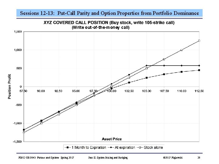
Sessions 12 -13: Put-Call Parity and Option Properties from Portfolio Dominance (Write out-of-the-money call) FINC-UB. 0043 Futures and Options Spring 2017 Part II: Option Pricing and Hedging © 2017 Figlewski 28

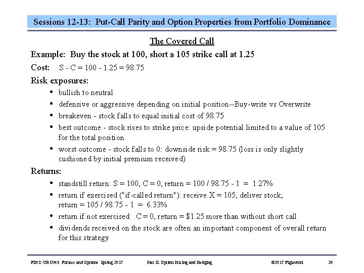
Sessions 12 -13: Put-Call Parity and Option Properties from Portfolio Dominance The Covered Call Example: Buy the stock at 100, short a 105 strike call at 1. 25 Cost: S - C = 100 - 1. 25 = 98. 75 Risk exposures: • • • bullish to neutral defensive or aggressive depending on initial position--Buy-write vs Overwrite breakeven - stock falls to equal initial cost of 98. 75 best outcome - stock rises to strike price: upside potential limited to a value of 105 for the total position worst outcome - stock falls to 0: downside risk = 98. 75 (loss is only slightly cushioned by initial premium received) Returns: • • standstill return: S = 100, C = 0, return = 100 / 98. 75 - 1 = 1. 27% return if exercised ("if-called return"): receive X = 105, deliver stock; return = 105 / 98. 75 - 1 = 6. 33% return if not exercised: C = 0, return = $1. 25 more than without short call dividends received on the stock are often an important component of overall return for this strategy FINC-UB. 0043 Futures and Options Spring 2017 Part II: Option Pricing and Hedging © 2017 Figlewski 29

Sessions 12 -13: Put-Call Parity and Option Properties from Portfolio Dominance FINC-UB. 0043 Futures and Options Spring 2017 Part II: Option Pricing and Hedging © 2017 Figlewski 30

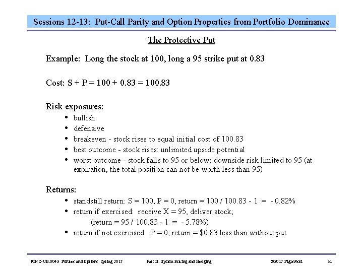
Sessions 12 -13: Put-Call Parity and Option Properties from Portfolio Dominance The Protective Put Example: Long the stock at 100, long a 95 strike put at 0. 83 Cost: S + P = 100 + 0. 83 = 100. 83 Risk exposures: • • • bullish. defensive breakeven - stock rises to equal initial cost of 100. 83 best outcome - stock rises: unlimited upside potential worst outcome - stock falls to 95 or below: downside risk limited to 95 (at expiration, the total position can not be worth less than 95) Returns: • • standstill return: S = 100, P = 0, return = 100 / 100. 83 - 1 = - 0. 82% return if exercised: receive X = 95, deliver stock; (return = 95 / 100. 83 - 1 = - 5. 78%) • return if not exercised: P = 0, return = $0. 83 less than without put FINC-UB. 0043 Futures and Options Spring 2017 Part II: Option Pricing and Hedging © 2017 Figlewski 31

Sessions 12 -13: Put-Call Parity and Option Properties from Portfolio Dominance A Very Important Arbitrage Trade Consider a call and a put on XYZ stock, with the same maturity, 1 month, and the same strike price, 100. (Both options are European. ) If XYZ is above 100 in a month, the 100 strike call will be exercised. If XYZ is below 100 in a month, the 100 strike put will be exercised. What if you buy the call and also write the put? • Suppose XYZ ends up at 105. You choose to exercise the call: you pay 100 and you get the stock. (The put is out of the money and expires without being exercised. ) • What if XYZ is at 95? The put will be exercised by your counterparty and you will have to buy the stock for 100. (The call is worthless. ) In other words, no matter what happens with the stock price, at maturity you will pay 100 and you will own the stock. FINC-UB. 0043 Futures and Options Spring 2017 Part II: Option Pricing and Hedging © 2017 Figlewski 32

Sessions 12 -13: Put-Call Parity and Option Properties from Portfolio Dominance Put-Call Parity This position returns exactly what you would have if you just bought the stock today, and financed a large part of the position by borrowing the present value of 100. (On option maturity day, you would own the stock and pay out 100. ) With two different ways to achieve exactly the same payoff, there is a possible arbitrage trade. If these two positions do not cost exactly the same to set up, arbitrageurs will buy the position in the way that is cheaper and sell it (i. e. , take the opposite position) in the way that is more expensive. The difference in cost between them is an arbitrage profit that is locked in. Trading will continue until prices come into line. In our example, arbitrage will force Call price - Put price = 100 - PV(100) The general Put-Call parity relationship that must hold in equilibrium is Call price - Put price C - P = = Asset price - PV(Strike price) S - PV ( X ) FINC-UB. 0043 Futures and Options Spring 2017 Part II: Option Pricing and Hedging © 2017 Figlewski 33

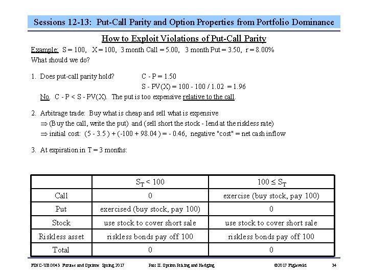
Sessions 12 -13: Put-Call Parity and Option Properties from Portfolio Dominance How to Exploit Violations of Put-Call Parity Example: S = 100, X = 100, 3 month Call = 5. 00, 3 month Put = 3. 50, r = 8. 00% What should we do? 1. Does put-call parity hold? C - P = 1. 50 S - PV(X) = 100 - 100 / 1. 02 = 1. 96 No. C - P < S - PV(X). The put is too expensive relative to the call. 2. Arbitrage trade: Buy what is cheap and sell what is expensive (Buy the call, write the put) and (sell short the stock - lend at the riskless rate) initial cost: (5 - 3. 5 ) + (-100 + 98. 04 ) = - 0. 46, negative "cost" = net cash inflow 3. At expiration in T = 3 months: ST < 100 ST Call 0 exercise (buy stock, pay 100) Put exercised (buy stock, pay 100) 0 Stock use stock to cover short sale Riskless asset riskless bonds pay off 100 Total 0 0 FINC-UB. 0043 Futures and Options Spring 2017 Part II: Option Pricing and Hedging © 2017 Figlewski 34

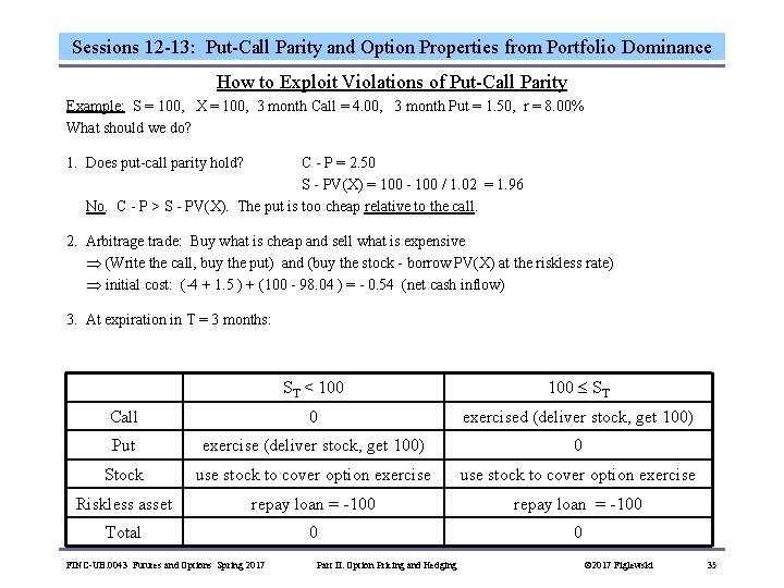
Sessions 12 -13: Put-Call Parity and Option Properties from Portfolio Dominance How to Exploit Violations of Put-Call Parity Example: S = 100, X = 100, 3 month Call = 4. 00, 3 month Put = 1. 50, r = 8. 00% What should we do? 1. Does put-call parity hold? C - P = 2. 50 S - PV(X) = 100 - 100 / 1. 02 = 1. 96 No. C - P > S - PV(X). The put is too cheap relative to the call. 2. Arbitrage trade: Buy what is cheap and sell what is expensive (Write the call, buy the put) and (buy the stock - borrow PV(X) at the riskless rate) initial cost: (-4 + 1. 5 ) + (100 - 98. 04 ) = - 0. 54 (net cash inflow) 3. At expiration in T = 3 months: ST < 100 ST Call 0 exercised (deliver stock, get 100) Put exercise (deliver stock, get 100) 0 Stock use stock to cover option exercise Riskless asset repay loan = -100 Total 0 0 FINC-UB. 0043 Futures and Options Spring 2017 Part II: Option Pricing and Hedging © 2017 Figlewski 35

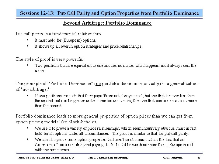
Sessions 12 -13: Put-Call Parity and Option Properties from Portfolio Dominance Beyond Arbitrage: Portfolio Dominance Put-call parity is a fundamental relationship. • • It must hold for (European) options. It shows up all over in option strategies and price relationships. The style of proof is very powerful. • Two positions that are equivalent to one another no matter what happens, must always cost the same. The principle of "Portfolio Dominance" (no portfolio dominance, actually) is a generalization of "no-arbitrage. " • If two positions are such that their payoffs are not always equal, but the first is never less than the second and can be greater under some circumstances, then the first position must cost more than the second. Portfolio dominance leads to more general properties of option prices than we can get from option pricing models like Black-Scholes. • • We use it to prove a variety of price relationships, which seem intuitively obvious, must in fact hold for all options under all circumstances. The proof is similar to that for put-call parity. We can also prove some option properties that aren't so obvious, such as the fact that an American call on a non-dividend paying stock should be worth no more than a European call with the same terms. FINC-UB. 0043 Futures and Options Spring 2017 Part II: Option Pricing and Hedging © 2017 Figlewski 36

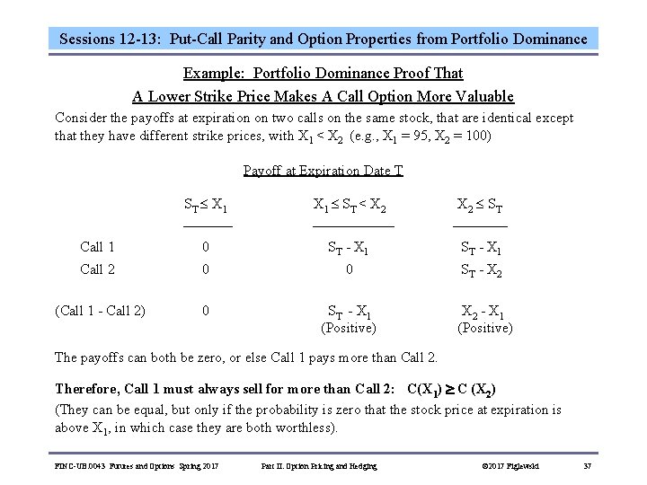
Sessions 12 -13: Put-Call Parity and Option Properties from Portfolio Dominance Example: Portfolio Dominance Proof That A Lower Strike Price Makes A Call Option More Valuable Consider the payoffs at expiration on two calls on the same stock, that are identical except that they have different strike prices, with X 1 < X 2 (e. g. , X 1 = 95, X 2 = 100) Payoff at Expiration Date T ST X 1 ST < X 2 ST Call 1 0 ST - X 1 Call 2 0 0 ST - X 2 (Call 1 - Call 2) 0 ST - X 1 (Positive) X 2 - X 1 (Positive) The payoffs can both be zero, or else Call 1 pays more than Call 2. Therefore, Call 1 must always sell for more than Call 2: C(X 1) C (X 2) (They can be equal, but only if the probability is zero that the stock price at expiration is above X 1, in which case they are both worthless). FINC-UB. 0043 Futures and Options Spring 2017 Part II: Option Pricing and Hedging © 2017 Figlewski 37

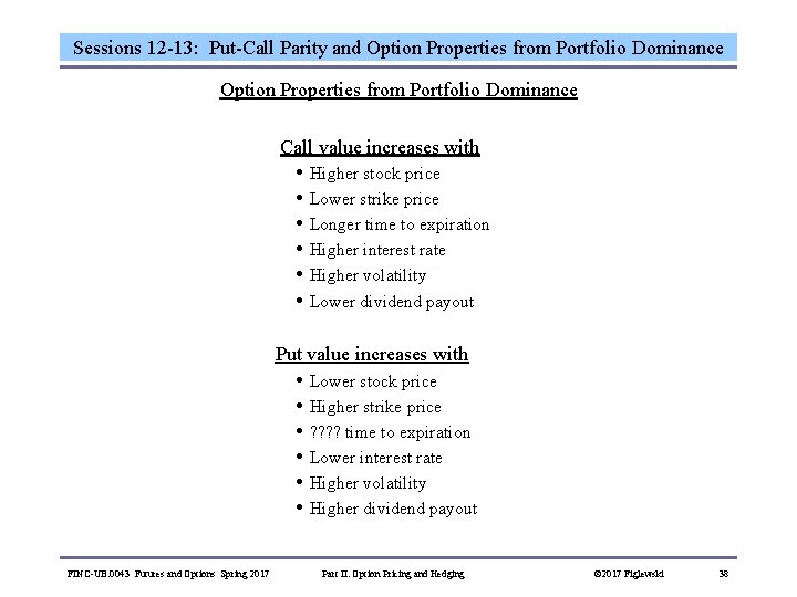
Sessions 12 -13: Put-Call Parity and Option Properties from Portfolio Dominance Call value increases with • Higher stock price • Lower strike price • Longer time to expiration • Higher interest rate • Higher volatility • Lower dividend payout Put value increases with • Lower stock price • Higher strike price • ? ? time to expiration • Lower interest rate • Higher volatility • Higher dividend payout FINC-UB. 0043 Futures and Options Spring 2017 Part II: Option Pricing and Hedging © 2017 Figlewski 38

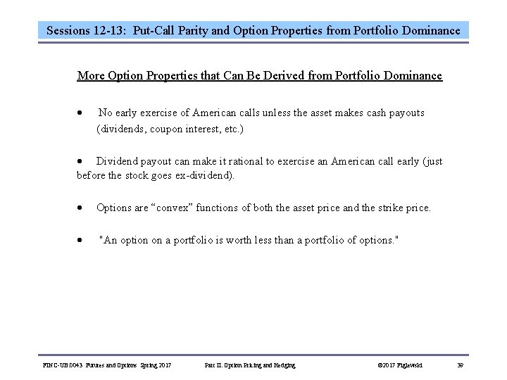
Sessions 12 -13: Put-Call Parity and Option Properties from Portfolio Dominance More Option Properties that Can Be Derived from Portfolio Dominance · No early exercise of American calls unless the asset makes cash payouts (dividends, coupon interest, etc. ) · Dividend payout can make it rational to exercise an American call early (just before the stock goes ex-dividend). · Options are “convex” functions of both the asset price and the strike price. · "An option on a portfolio is worth less than a portfolio of options. " FINC-UB. 0043 Futures and Options Spring 2017 Part II: Option Pricing and Hedging © 2017 Figlewski 39

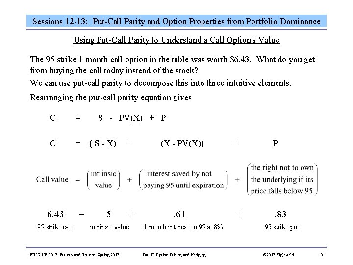
Sessions 12 -13: Put-Call Parity and Option Properties from Portfolio Dominance Using Put-Call Parity to Understand a Call Option's Value The 95 strike 1 month call option in the table was worth $6. 43. What do you get from buying the call today instead of the stock? We can use put-call parity to decompose this into three intuitive elements. Rearranging the put-call parity equation gives C = S - PV(X) + P C = ( S - X) + (X - PV(X)) + P 6. 43 = 5 + . 61 + . 83 95 strike call intrinsic value 1 month interest on 95 at 8% 95 strike put FINC-UB. 0043 Futures and Options Spring 2017 Part II: Option Pricing and Hedging © 2017 Figlewski 40

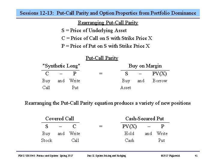
Sessions 12 -13: Put-Call Parity and Option Properties from Portfolio Dominance Rearranging Put-Call Parity S = Price of Underlying Asset C = Price of Call on S with Strike Price X P = Price of Put on S with Strike Price X Put-Call Parity "Synthetic Long" Buy on Margin C – P = S – PV(X) Buy and Write Buy and Borrow Call Put Asset Rearranging the Put-Call Parity equation produces a variety of new positions Covered Call Cash-Secured Put S – C = PV(X) – P Buy and Write Hold and Write Stock Call Cash Put FINC-UB. 0043 Futures and Options Spring 2017 Part II: Option Pricing and Hedging © 2017 Figlewski 41

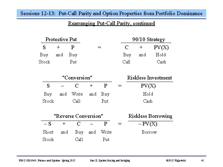
Sessions 12 -13: Put-Call Parity and Option Properties from Portfolio Dominance Rearranging Put-Call Parity, continued Protective Put 90/10 Strategy S + P = C + PV(X) Buy and Buy Buy and Hold Stock Put Call Cash "Conversion" Riskless Investment S – C + P = PV(X) Buy and Write and Buy Hold Stock Call Put Cash "Reverse Conversion" Riskless Borrowing – S + C – P = – PV(X) Short and Buy and Write Borrow Stock Call Put FINC-UB. 0043 Futures and Options Spring 2017 Part II: Option Pricing and Hedging © 2017 Figlewski 42

Session 14 -16: Option Pricing Models: The Binomial Model and Black-Scholes Option Pricing Models Option properties derived from portfolio dominance are very general, but not very precise. Many people tried to find a pricing formula that could say exactly how many dollars a given option is worth. But for years, no one succeeded. Fischer Black and Myron Scholes, along with Robert Merton, did it in the early 1970 s, using a kind of mathematics borrowed from physics to model the behavior of stock prices. The new theory was very hard to explain to students (or to finance professors). Just for pedagogical purposes, in his 1977 Investments textbook, William Sharpe introduced the Binomial model, a very simplified framework in which an option could be easily understood and priced. However, it turned out that the simple classroom model could be developed into an extremely powerful and practical valuation tool, with flexibility to solve some kinds of problems, like pricing an American put, that the Black-Scholes model can not handle. It has been successfully extended to Trinomial and more complicated lattices for even more power and flexibility. We start with the Binomial in this session and move on to the Black-Scholes model in the next one. FINC-UB. 0043 Futures and Options Spring 2017 Part II: Option Pricing and Hedging © 2017 Figlewski 43

Session 14 -16: Option Pricing Models: The Binomial Model and Black-Scholes Theoretical Underpinning of Derivatives Pricing Models There are two types of valuation models for securities in modern finance theory, Equilibrium models and Arbitrage-based models. We have seen this already for futures. • • The Expectations Model is an equilibrium model. So is the Capital Asset Pricing Model. The Cost of Carry Model is an arbitrage-based model. Equilibrium Models • • • The security price is determined by aggregate supply and demand in the market. The model value for a security should include a risk premium Investors value each security relative to the entire set of available instruments. Prices are brought into line with theoretical values because investors search out undervalued securities and bid up their prices. They sell off overvalued securities, driving their prices down until they become cheap enough to be worth holding. All securities must be in equilibrium for the model to apply. FINC-UB. 0043 Futures and Options Spring 2017 Part II: Option Pricing and Hedging © 2017 Figlewski 44

Session 14 -16: Option Pricing Models: The Binomial Model and Black-Scholes Theoretical Underpinning of Derivatives Pricing Models, p. 2 Arbitrage-Based Models • • • The price is determined by the possibility of arbitrage between the derivative security and its underlying asset. The derivative is only valued relative to its underlying (and the riskless interest rate) The model price does not include a risk premium. All investors should value the security the same way regardless of how risk averse or risk tolerant they are. Prices are brought into line by arbitrage. In theory, because mispricing creates the opportunity for riskless arbitrage, it only takes a single energetic arbitrageur to force the market price to the model value. Because the model only says how the derivative should be priced relative to the underlying, it doesn't matter whether the underlying or any other security is in equilibrium with respect to other traded assets. Examples: The Binomial Model, the Black-Scholes Model, and the Cost of Carry Model for futures FINC-UB. 0043 Futures and Options Spring 2017 Part II: Option Pricing and Hedging © 2017 Figlewski 45

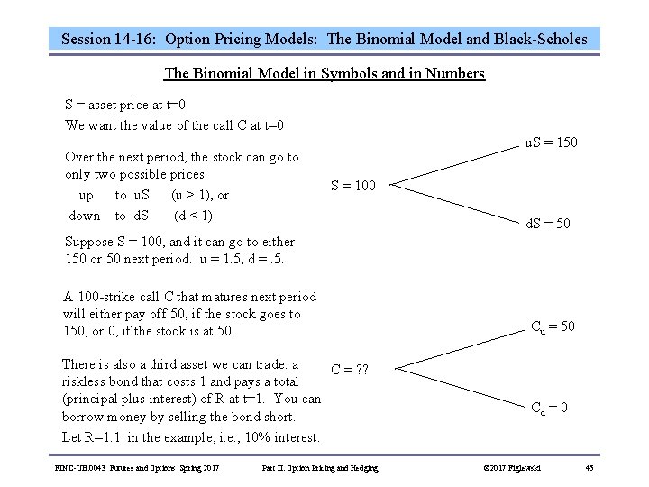
Session 14 -16: Option Pricing Models: The Binomial Model and Black-Scholes The Binomial Model in Symbols and in Numbers S = asset price at t=0. We want the value of the call C at t=0 Over the next period, the stock can go to only two possible prices: up to u. S (u > 1), or down to d. S (d < 1). u. S = 150 S = 100 d. S = 50 Suppose S = 100, and it can go to either 150 or 50 next period. u = 1. 5, d =. 5. A 100 -strike call C that matures next period will either pay off 50, if the stock goes to 150, or 0, if the stock is at 50. There is also a third asset we can trade: a C = ? ? riskless bond that costs 1 and pays a total (principal plus interest) of R at t=1. You can borrow money by selling the bond short. Let R=1. 1 in the example, i. e. , 10% interest. Cu = 50 Cd = 0 FINC-UB. 0043 Futures and Options Spring 2017 Part II: Option Pricing and Hedging © 2017 Figlewski 46

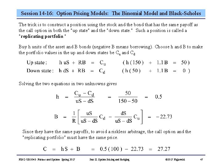
Session 14 -16: Option Pricing Models: The Binomial Model and Black-Scholes The trick is to construct a position using the stock and the bond that has the same payoff as the call option in both the "up state" and the "down state. " Such a position is called a "replicating portfolio. " Buy h units of the asset and B bonds (negative B means borrowing). Choose h and B to make the portfolio values in the up and down states be Cu and Cd. Solving the two equations in two unknowns gives Since they have the same payoffs, to avoid a riskless arbitrage, the call option and the "replicating portfolio" must have the same price. FINC-UB. 0043 Futures and Options Spring 2017 Part II: Option Pricing and Hedging © 2017 Figlewski 47

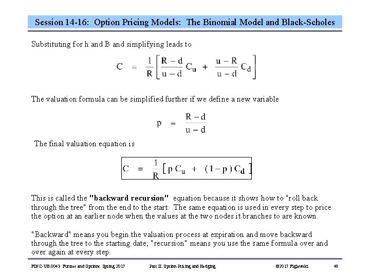
Session 14 -16: Option Pricing Models: The Binomial Model and Black-Scholes Substituting for h and B and simplifying leads to The valuation formula can be simplified further if we define a new variable The final valuation equation is This is called the "backward recursion" equation because it shows how to "roll back through the tree" from the end to the start. The same equation is used in every step to price the option at an earlier node when the values at the two nodes it branches to are known. "Backward" means you begin the valuation process at expiration and move backward through the tree to the starting date; "recursion" means you use the same formula over and over again at every step. FINC-UB. 0043 Futures and Options Spring 2017 Part II: Option Pricing and Hedging © 2017 Figlewski 48

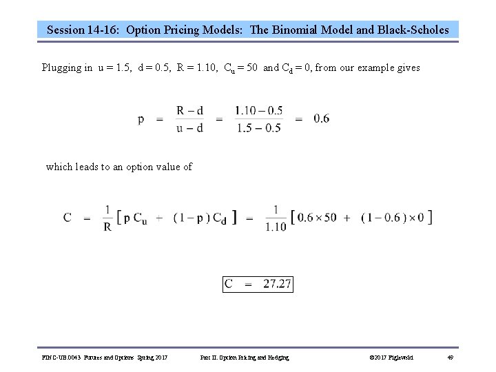
Session 14 -16: Option Pricing Models: The Binomial Model and Black-Scholes Plugging in u = 1. 5, d = 0. 5, R = 1. 10, Cu = 50 and Cd = 0, from our example gives which leads to an option value of FINC-UB. 0043 Futures and Options Spring 2017 Part II: Option Pricing and Hedging © 2017 Figlewski 49

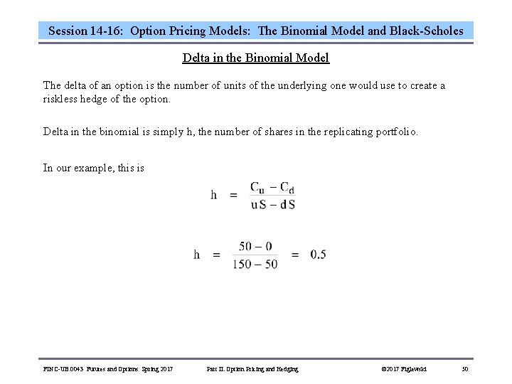
Session 14 -16: Option Pricing Models: The Binomial Model and Black-Scholes Delta in the Binomial Model The delta of an option is the number of units of the underlying one would use to create a riskless hedge of the option. Delta in the binomial is simply h, the number of shares in the replicating portfolio. In our example, this is FINC-UB. 0043 Futures and Options Spring 2017 Part II: Option Pricing and Hedging © 2017 Figlewski 50

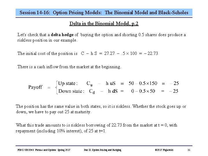
Session 14 -16: Option Pricing Models: The Binomial Model and Black-Scholes Delta in the Binomial Model, p. 2 Let's check that a delta hedge of buying the option and shorting 0. 5 shares does produce a riskless position in our example. The initial cost of the position is C – h S = 27. 27 – . 5 100 = – 22. 73 There is a cash inflow from the market at the beginning. The position has the same value in both states, so it is riskless. Whether the stock goes up or down, we have to pay out 25 at maturity. What this trade amounts to is riskless borrowing of 22. 73 from the market at t = 0, with repayment (including 10% interest), of 25 at t=1. FINC-UB. 0043 Futures and Options Spring 2017 Part II: Option Pricing and Hedging © 2017 Figlewski 51

Session 14 -16: Option Pricing Models: The Binomial Model and Black-Scholes Two Important Properties of the Binomial Model 1. The backward recursion valuation method works essentially the same way for any contingent claim within the binomial framework. There is nothing in the way the pricing equation was derived that limits it to calls. 2. The valuation equation does not involve the probabilities attached to the up and down branches. The option value is the same for all probabilities. (The replicating portfolio matches the option value in both possible states, so it doesn't matter how likely each one is. ) FINC-UB. 0043 Futures and Options Spring 2017 Part II: Option Pricing and Hedging © 2017 Figlewski 52

Session 14 -16: Option Pricing Models: The Binomial Model and Black-Scholes Risk Neutral Valuation Recall the Cost of Carry model for pricing gold futures. If S is the spot price for gold, say $1600 per ounce, and r is the riskless interest rate, say 10%, what should the futures price be for a 1 year futures contract? F 1 year = S ( 1 + r T/365) = 1600 x 1. 10 = 1760 Suppose investors are so risk averse that they only hold gold if they expect the price to go up 25% a year. For them to pay $1600 an ounce for gold today, investors must be expecting it to go up to 1600 x 1. 25 = $2000 an ounce next year. What is the equilibrium gold futures price in that case? It is the same 1760! The gold futures market obeys the cost of carry model because you can buy gold and hedge away all the risk with futures, leaving a riskless position that must earn the riskless interest rate, no matter how risk averse investors are. Suppose investors are completely indifferent to risk: They are "risk neutral. " Then any asset, risky or not, should be priced to earn the same expected return. If gold is at 1600 in the spot market when investors are risk-neutral, it is because the market expects the price to go up to 1600 x 1. 10 = $1760 next year. What is the futures price? Still 1760, of course. But now, the cost of carry model and the expectations model give the same answer. "Risk neutral valuation" means the derivatives price in an arbitrage-based model is the same as what it would be in the expectations model in a world of risk neutral investors. FINC-UB. 0043 Futures and Options Spring 2017 Part II: Option Pricing and Hedging © 2017 Figlewski 53

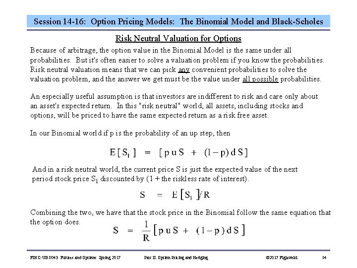
Session 14 -16: Option Pricing Models: The Binomial Model and Black-Scholes Risk Neutral Valuation for Options Because of arbitrage, the option value in the Binomial Model is the same under all probabilities. But it's often easier to solve a valuation problem if you know the probabilities. Risk neutral valuation means that we can pick any convenient probabilities to solve the valuation problem, and the answer we get must be the value under all possible probabilities. An especially useful assumption is that investors are indifferent to risk and care only about an asset's expected return. In this "risk neutral" world, all assets, including stocks and options, will be priced to have the same expected return as a risk free asset. In our Binomial world if p is the probability of an up step, then And in a risk neutral world, the current price S is just the expected value of the next period stock price S 1 discounted by (1 + the riskless rate of interest). Combining the two, we have that the stock price in the Binomial follow the same equation that the option does. FINC-UB. 0043 Futures and Options Spring 2017 Part II: Option Pricing and Hedging © 2017 Figlewski 54

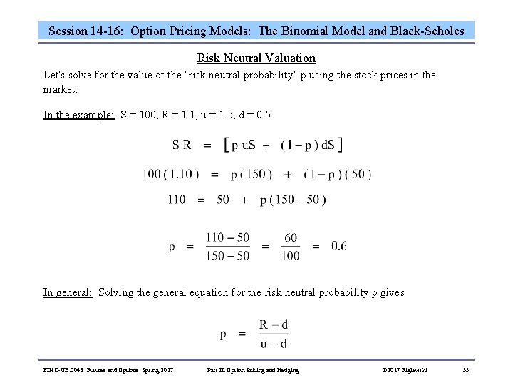
Session 14 -16: Option Pricing Models: The Binomial Model and Black-Scholes Risk Neutral Valuation Let's solve for the value of the "risk neutral probability" p using the stock prices in the market. In the example: S = 100, R = 1. 1, u = 1. 5, d = 0. 5 In general: Solving the general equation for the risk neutral probability p gives FINC-UB. 0043 Futures and Options Spring 2017 Part II: Option Pricing and Hedging © 2017 Figlewski 55

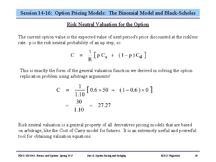
Session 14 -16: Option Pricing Models: The Binomial Model and Black-Scholes Risk Neutral Valuation for the Option The current option value is the expected value of next period's price discounted at the riskless rate. p is the risk neutral probability of an up step, so This is exactly the form of the general valuation function we derived in solving the option replication problem using arbitrage arguments! Risk neutral valuation is a general property of all derivatives pricing models that are based on arbitrage, like the Cost of Carry model for futures. It is an extremely useful and powerful tool for obtaining valuation equations. FINC-UB. 0043 Futures and Options Spring 2017 Part II: Option Pricing and Hedging © 2017 Figlewski 56

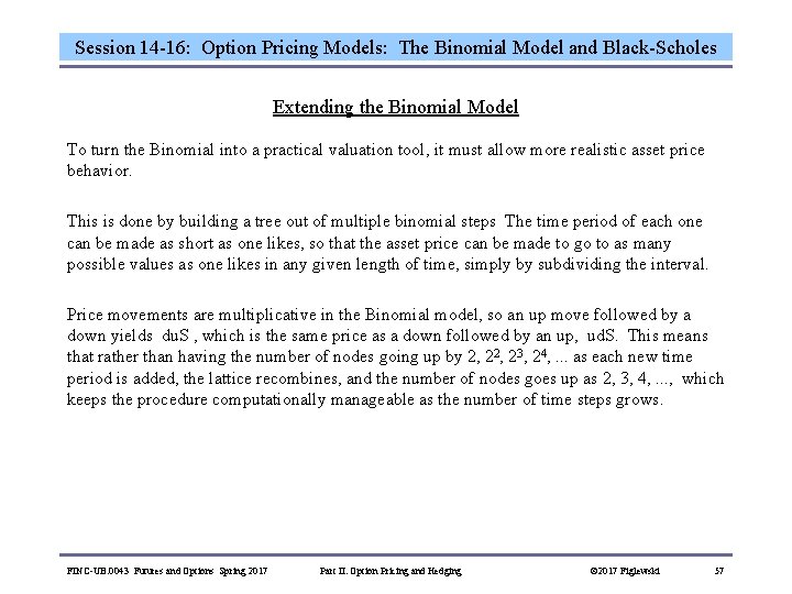
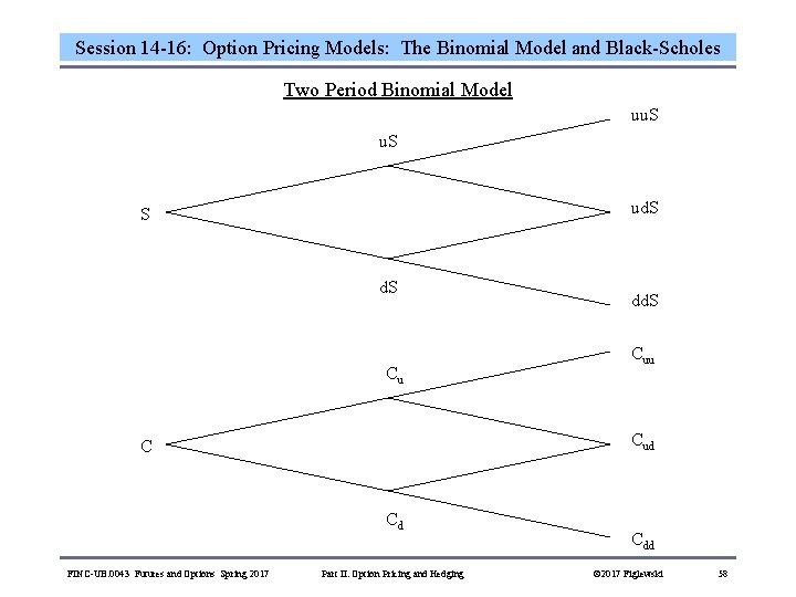
Session 14 -16: Option Pricing Models: The Binomial Model and Black-Scholes Extending the Binomial Model To turn the Binomial into a practical valuation tool, it must allow more realistic asset price behavior. This is done by building a tree out of multiple binomial steps The time period of each one can be made as short as one likes, so that the asset price can be made to go to as many possible values as one likes in any given length of time, simply by subdividing the interval. Price movements are multiplicative in the Binomial model, so an up move followed by a down yields du. S , which is the same price as a down followed by an up, ud. S. This means that rather than having the number of nodes going up by 2, 23, 24, . . . as each new time period is added, the lattice recombines, and the number of nodes goes up as 2, 3, 4, . . . , which keeps the procedure computationally manageable as the number of time steps grows. FINC-UB. 0043 Futures and Options Spring 2017 Part II: Option Pricing and Hedging © 2017 Figlewski 57

Session 14 -16: Option Pricing Models: The Binomial Model and Black-Scholes Two Period Binomial Model uu. S ud. S S d. S Cu dd. S Cuu Cud C Cd Cdd FINC-UB. 0043 Futures and Options Spring 2017 Part II: Option Pricing and Hedging © 2017 Figlewski 58

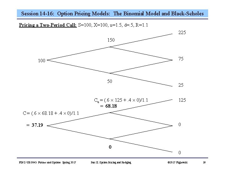
Session 14 -16: Option Pricing Models: The Binomial Model and Black-Scholes Pricing a Two-Period Call: S=100, X=100, u=1. 5, d=. 5, R=1. 1 225 150 75 100 50 Cu = (. 6 125 +. 4 0)/1. 1 = 68. 18 25 125 C = (. 6 68. 18 +. 4 0)/1. 1 0 = 37. 19 0 0 FINC-UB. 0043 Futures and Options Spring 2017 Part II: Option Pricing and Hedging © 2017 Figlewski 59

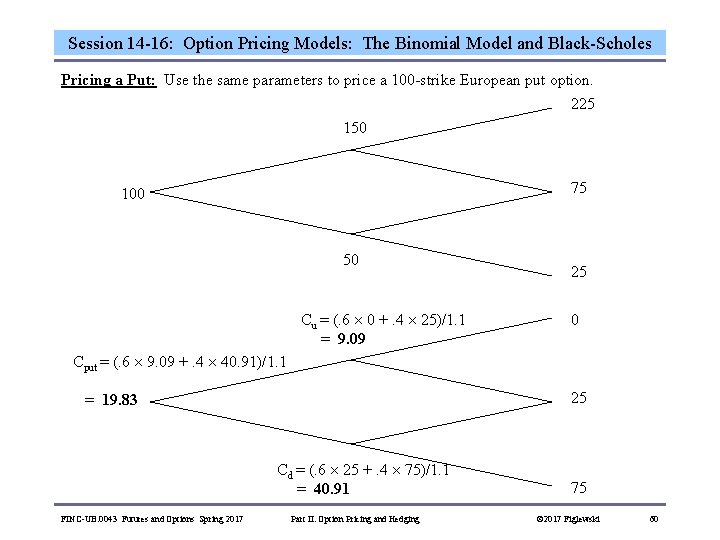
Session 14 -16: Option Pricing Models: The Binomial Model and Black-Scholes Pricing a Put: Use the same parameters to price a 100 -strike European put option. 225 150 75 100 50 Cu = (. 6 0 +. 4 25)/1. 1 = 9. 09 25 0 Cput = (. 6 9. 09 +. 4 40. 91)/1. 1 25 = 19. 83 Cd = (. 6 25 +. 4 75)/1. 1 = 40. 91 75 FINC-UB. 0043 Futures and Options Spring 2017 Part II: Option Pricing and Hedging © 2017 Figlewski 60

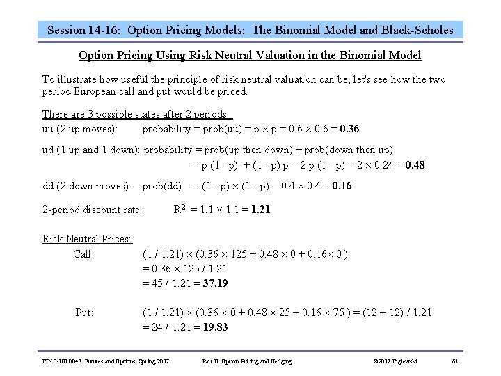
Session 14 -16: Option Pricing Models: The Binomial Model and Black-Scholes Option Pricing Using Risk Neutral Valuation in the Binomial Model To illustrate how useful the principle of risk neutral valuation can be, let's see how the two period European call and put would be priced. There are 3 possible states after 2 periods: uu (2 up moves): probability = prob(uu) = p p = 0. 6 = 0. 36 ud (1 up and 1 down): probability = prob(up then down) + prob(down then up) = p (1 - p) + (1 - p) p = 2 p (1 - p) = 2 0. 24 = 0. 48 dd (2 down moves): prob(dd) = (1 - p) = 0. 4 = 0. 16 2 -period discount rate: R 2 = 1. 1 = 1. 21 Risk Neutral Prices: Call: (1 / 1. 21) (0. 36 125 + 0. 48 0 + 0. 16 0 ) = 0. 36 125 / 1. 21 = 45 / 1. 21 = 37. 19 Put: (1 / 1. 21) (0. 36 0 + 0. 48 25 + 0. 16 75 ) = (12 + 12) / 1. 21 = 24 / 1. 21 = 19. 83 FINC-UB. 0043 Futures and Options Spring 2017 Part II: Option Pricing and Hedging © 2017 Figlewski 61

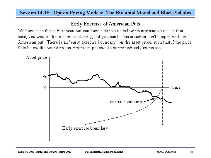
Session 14 -16: Option Pricing Models: The Binomial Model and Black-Scholes Early Exercise of American Puts We have seen that a European put can have a fair value below its intrinsic value. In that case, you would like to exercise it early, but you can't. This situation can't happen with an American put. There is an "early exercise boundary" on the asset price, such that if the price falls below the boundary, an American put should be immediately exercised. Asset price S 0 T time X exercise put here Early exercise boundary FINC-UB. 0043 Futures and Options Spring 2017 Part II: Option Pricing and Hedging © 2017 Figlewski 62

Session 14 -16: Option Pricing Models: The Binomial Model and Black-Scholes Early Exercise of American Puts It is rational to exercise an American put early. Time value has two components, one due to "optionality" and the other due to the interest that can be earned on the exercise price. These are both positive for a call option, so you won't exercise early. Optionality is also positive for a put, but the interest effect is negative: If you are going to exercise the option and receive the exercise price in cash, the longer you have to wait, the smaller is the present value of that cash. Time value goes to zero for a deep in the money put, at which point it is better to exercise it than to hold it any longer. An American put is therefore worth more than a European put, because early exercise has economic value. But valuing the early exercise feature of an American put is mathematically tricky, so that there is no "simple" closed-formula for the American put price. Put exercise is more likely with • high intrinsic value, X - S • short time to maturity • low volatility • high interest rate • high dividend yield (payment of a dividend tends to delay exercise until after exdividend date) FINC-UB. 0043 Futures and Options Spring 2017 Part II: Option Pricing and Hedging © 2017 Figlewski 63

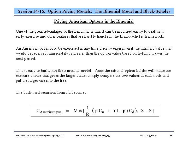
Session 14 -16: Option Pricing Models: The Binomial Model and Black-Scholes Pricing American Options in the Binomial One of the great advantages of the Binomial is that it can be modified easily to deal with early exercise and other features that are hard to handle in the Black-Scholes framework. An American put should be exercised at any time prior to expiration if the intrinsic value that would be received immediately is greater than the option value based on holding it over the next period. This is easy to build into the Binomial model. Since the rational option holder will make the exercise choice that gives the larger value, simply compare the two values at each node and put the larger one into the tree. The backward recursion formula becomes FINC-UB. 0043 Futures and Options Spring 2017 Part II: Option Pricing and Hedging © 2017 Figlewski 64

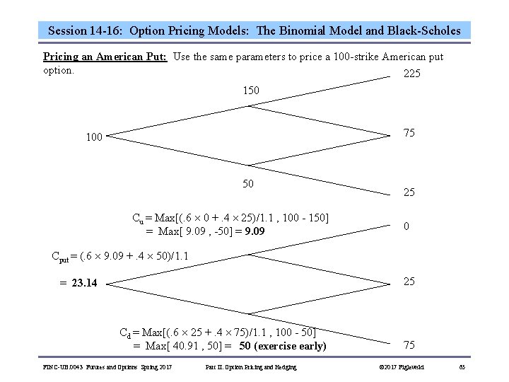
Session 14 -16: Option Pricing Models: The Binomial Model and Black-Scholes Pricing an American Put: Use the same parameters to price a 100 -strike American put option. 225 150 75 100 50 Cu = Max[(. 6 0 +. 4 25)/1. 1 , 100 - 150] = Max[ 9. 09 , -50] = 9. 09 25 0 Cput = (. 6 9. 09 +. 4 50)/1. 1 25 = 23. 14 Cd = Max[(. 6 25 +. 4 75)/1. 1 , 100 - 50] = Max[ 40. 91 , 50] = 50 (exercise early) 75 FINC-UB. 0043 Futures and Options Spring 2017 Part II: Option Pricing and Hedging © 2017 Figlewski 65

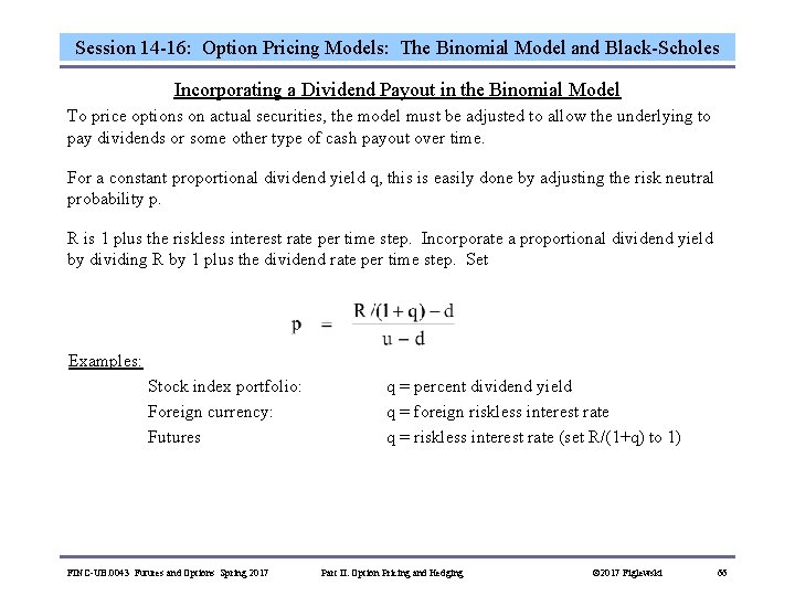
Session 14 -16: Option Pricing Models: The Binomial Model and Black-Scholes Incorporating a Dividend Payout in the Binomial Model To price options on actual securities, the model must be adjusted to allow the underlying to pay dividends or some other type of cash payout over time. For a constant proportional dividend yield q, this is easily done by adjusting the risk neutral probability p. R is 1 plus the riskless interest rate per time step. Incorporate a proportional dividend yield by dividing R by 1 plus the dividend rate per time step. Set Examples: Stock index portfolio: Foreign currency: Futures q = percent dividend yield q = foreign riskless interest rate q = riskless interest rate (set R/(1+q) to 1) FINC-UB. 0043 Futures and Options Spring 2017 Part II: Option Pricing and Hedging © 2017 Figlewski 66

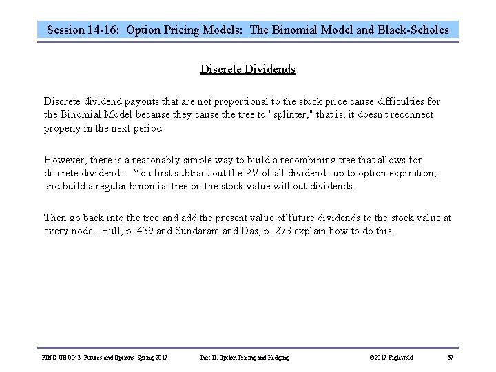
Session 14 -16: Option Pricing Models: The Binomial Model and Black-Scholes Discrete Dividends Discrete dividend payouts that are not proportional to the stock price cause difficulties for the Binomial Model because they cause the tree to "splinter, " that is, it doesn't reconnect properly in the next period. However, there is a reasonably simple way to build a recombining tree that allows for discrete dividends. You first subtract out the PV of all dividends up to option expiration, and build a regular binomial tree on the stock value without dividends. Then go back into the tree and add the present value of future dividends to the stock value at every node. Hull, p. 439 and Sundaram and Das, p. 273 explain how to do this. FINC-UB. 0043 Futures and Options Spring 2017 Part II: Option Pricing and Hedging © 2017 Figlewski 67

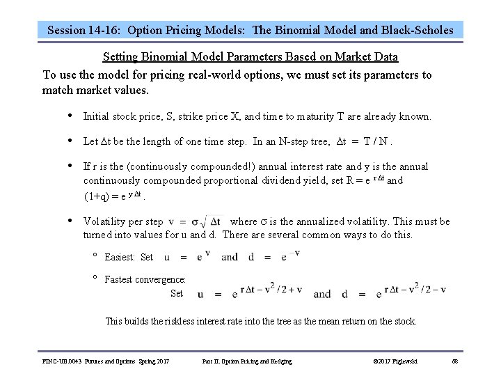
Session 14 -16: Option Pricing Models: The Binomial Model and Black-Scholes Setting Binomial Model Parameters Based on Market Data To use the model for pricing real-world options, we must set its parameters to match market values. • Initial stock price, S, strike price X, and time to maturity T are already known. • Let t be the length of one time step. In an N-step tree, t = T / N. • If r is the (continuously compounded!) annual interest rate and y is the annual continuously compounded proportional dividend yield, set R = e r t and (1+q) = e y t. • Volatility per step where is the annualized volatility. This must be turned into values for u and d. There are several common ways to do this. ° Easiest: Set ° Fastest convergence: Set This builds the riskless interest rate into the tree as the mean return on the stock. FINC-UB. 0043 Futures and Options Spring 2017 Part II: Option Pricing and Hedging © 2017 Figlewski 68

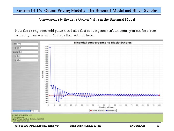
Session 14 -16: Option Pricing Models: The Binomial Model and Black-Scholes The Binomial model allows us to approximate option values to as close a degree of accuracy as we want. It is also much more flexible than Black-Scholes, so it can be used to solve many valuation problems, such as pricing an American put, that the Black-Scholes model can't handle. However, the Binomial is just an approximation, not a "closed-form" solution. A closed form solution is an equation that gives the exact option value as a function of a set of input parameters. Also, the Binomial is less efficient than a closed-form equation. It may take a long time to converge to the exact option value as the number of time steps in the tree is increased, and convergence is not monotonic (for example, a 200 step tree may give a less accurate answer than a 100 step tree). This session introduces the Black-Scholes model. This classic model is a closed-form solution to the option pricing problem. It is universally used in practice (although not in the way theory says it should be used) and it points the way towards similar valuation equations for other types of derivative instruments with option features. FINC-UB. 0043 Futures and Options Spring 2017 Part II: Option Pricing and Hedging © 2017 Figlewski 69

Session 14 -16: Option Pricing Models: The Binomial Model and Black-Scholes Convergence to the True Option Value in the Binomial Model Note the strong even-odd pattern and also that convergence isn't uniform: you can be closer to the right answer with 50 steps than with 80 here. FINC-UB. 0043 Futures and Options Spring 2017 Part II: Option Pricing and Hedging © 2017 Figlewski 70

Session 14 -16: Option Pricing Models: The Binomial Model and Black-Scholes Dynamic Hedging to Replicate Option Payoffs The Binomial Model set up a framework in which the underlying asset and the riskless bond could be combined to create a position that exactly replicates the payoff on the option. The Black-Scholes model is derived in a similar way: The option and the stock are combined to create a hedged position that is like a riskless bond. Like the bond, the riskless option-stock hedged position must return the riskless rate of interest. This leads to a fair price for the option. Black and Scholes' assumptions permit a much more realistic price process than the Binomial for the underlying asset, while still allowing a riskless hedge to be constructed over the option's entire lifetime. However, this requires a dynamic hedging strategy, because the position is only riskless over the next instant in time, and then it must be rebalanced. FINC-UB. 0043 Futures and Options Spring 2017 Part II: Option Pricing and Hedging © 2017 Figlewski 71

Session 14 -16: Option Pricing Models: The Binomial Model and Black-Scholes Underlying Assumptions of the Black-Scholes Option Pricing Model • Options are European • "Perfect" markets -- no transactions costs, no taxes, no constraints on short selling with full use of the proceeds, no indivisibilities, etc. • No limits on borrowing or lending at a known risk free rate of interest • The price of the underlying asset follows a "lognormal diffusion" process • The return volatility of the underlying asset is known • No dividends or cash payouts from the underlying asset prior to option maturity FINC-UB. 0043 Futures and Options Spring 2017 Part II: Option Pricing and Hedging © 2017 Figlewski 72

Session 14 -16: Option Pricing Models: The Binomial Model and Black-Scholes The Asset Price Process The Black-Scholes model assumes the price of the underlying asset, S, follows a "lognormal diffusion" process: d. S = S dt + S dz where d. S = the change in stock price over the next instant = the "drift, " that is, the average rate of capital gains as a continuously compounded annualized figure dt = an "instant" = the volatility, expressed as an annual rate dz = "Brownian motion, " a very small random shock to the price over the next instant. dz has mean zero and variance 1 dt. The standard deviation of dz is (which is a lot bigger than dt when dt is very small. This means the volatility term dominates the drift term over short time periods. ) Current dz is independent of all dz in previous periods FINC-UB. 0043 Futures and Options Spring 2017 Part II: Option Pricing and Hedging © 2017 Figlewski 73

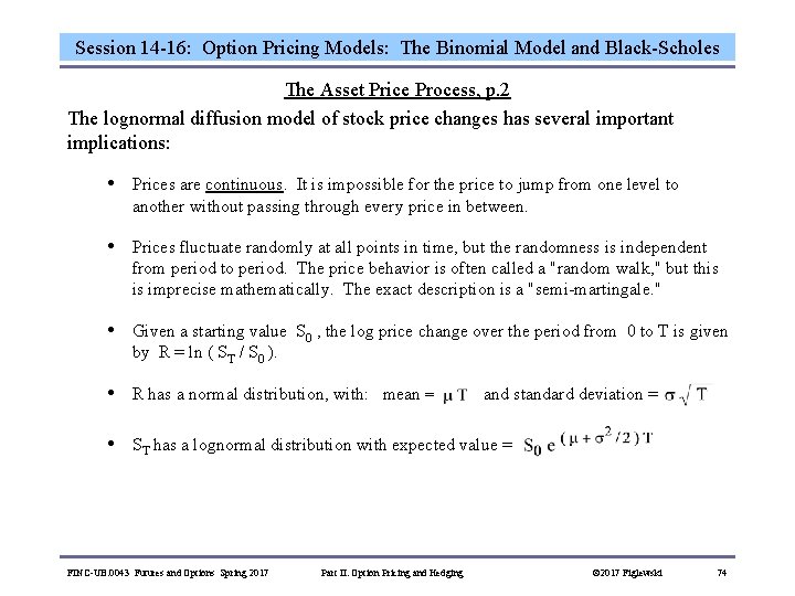
Session 14 -16: Option Pricing Models: The Binomial Model and Black-Scholes The Asset Price Process, p. 2 The lognormal diffusion model of stock price changes has several important implications: • Prices are continuous. It is impossible for the price to jump from one level to another without passing through every price in between. • Prices fluctuate randomly at all points in time, but the randomness is independent from period to period. The price behavior is often called a "random walk, " but this is imprecise mathematically. The exact description is a "semi-martingale. " • Given a starting value S 0 , the log price change over the period from 0 to T is given by R = ln ( ST / S 0 ). • R has a normal distribution, with: mean = and standard deviation = • ST has a lognormal distribution with expected value = FINC-UB. 0043 Futures and Options Spring 2017 Part II: Option Pricing and Hedging © 2017 Figlewski 74

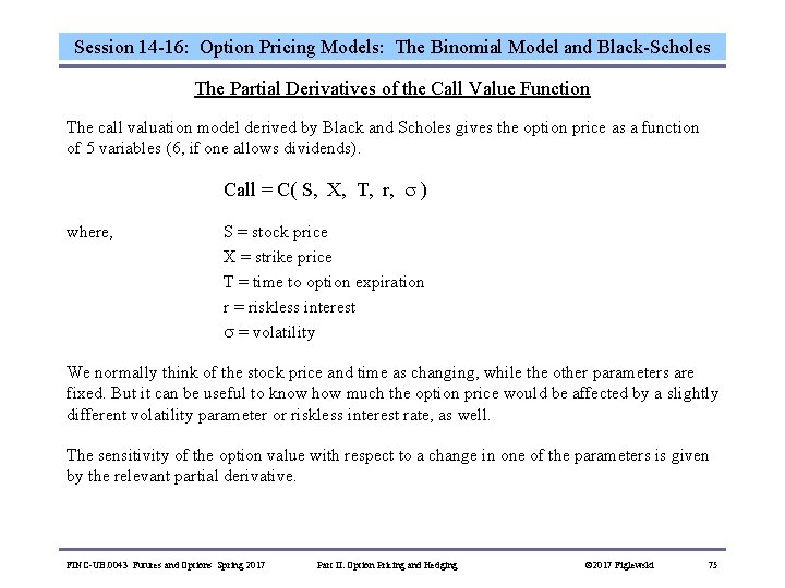
Session 14 -16: Option Pricing Models: The Binomial Model and Black-Scholes The Partial Derivatives of the Call Value Function The call valuation model derived by Black and Scholes gives the option price as a function of 5 variables (6, if one allows dividends). Call = C( S, X, T, r, ) where, S = stock price X = strike price T = time to option expiration r = riskless interest = volatility We normally think of the stock price and time as changing, while the other parameters are fixed. But it can be useful to know how much the option price would be affected by a slightly different volatility parameter or riskless interest rate, as well. The sensitivity of the option value with respect to a change in one of the parameters is given by the relevant partial derivative. FINC-UB. 0043 Futures and Options Spring 2017 Part II: Option Pricing and Hedging © 2017 Figlewski 75

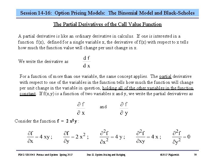
Session 14 -16: Option Pricing Models: The Binomial Model and Black-Scholes The Partial Derivatives of the Call Value Function A partial derivative is like an ordinary derivative in calculus. If one is interested in a function f(x), defined for a single variable x, the derivative of f(x) with respect to x tells how much the function value will change per unit change in x. We write the derivative as For a function of more than one variable, the same concept applies. The partial derivative with respect to one of the variables in the function tells how much the function will change per unit change in the variable in question, holding all of the other variables in the function constant. If f(x, y) is a function of two variables x and y, we write the partial derivatives as and Consider the function f = 2 x 2 y : FINC-UB. 0043 Futures and Options Spring 2017 Part II: Option Pricing and Hedging © 2017 Figlewski 76

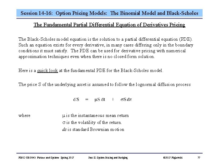
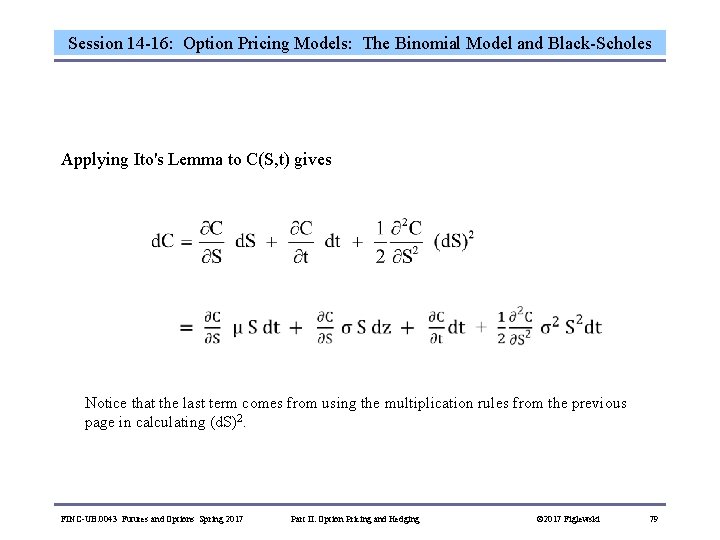
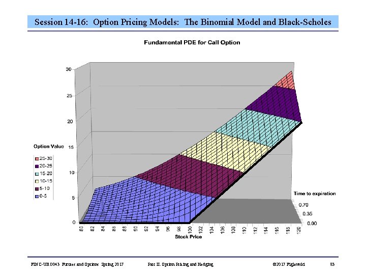
Session 14 -16: Option Pricing Models: The Binomial Model and Black-Scholes The Fundamental Partial Differential Equation of Derivatives Pricing The Black-Scholes model equation is the solution to a partial differential equation (PDE). Such an equation exists for every derivative, in many cases differing only in the boundary conditions it must satisfy. The PDE can be used for derivative pricing with numerical approximation techniques even when there is no closed form solution. Here is a quick look at the fundamental PDE for the Black-Scholes model. The price S of the underlying asset is assumed to follow the lognormal diffusion process where is the instantaneous mean return is the volatility of the return. dz is standard Brownian motion FINC-UB. 0043 Futures and Options Spring 2017 Part II: Option Pricing and Hedging © 2017 Figlewski 77

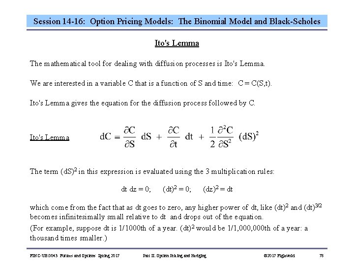
Session 14 -16: Option Pricing Models: The Binomial Model and Black-Scholes Ito's Lemma The mathematical tool for dealing with diffusion processes is Ito's Lemma. We are interested in a variable C that is a function of S and time: C = C(S, t). Ito's Lemma gives the equation for the diffusion process followed by C. Ito's Lemma The term (d. S)2 in this expression is evaluated using the 3 multiplication rules: dt dz = 0; (dt)2 = 0; (dz)2 = dt which come from the fact that as dt goes to zero, any higher power of dt, like (dt)2 and (dt)3/2 becomes infinitesimally small relative to dt and drops out of the equation. (For example, suppose dt is 1/1000 th of a year. (dt)2 would be 1/1, 000 th of a year: a thousand times smaller. ) FINC-UB. 0043 Futures and Options Spring 2017 Part II: Option Pricing and Hedging © 2017 Figlewski 78

Session 14 -16: Option Pricing Models: The Binomial Model and Black-Scholes Applying Ito's Lemma to C(S, t) gives Notice that the last term comes from using the multiplication rules from the previous page in calculating (d. S)2. FINC-UB. 0043 Futures and Options Spring 2017 Part II: Option Pricing and Hedging © 2017 Figlewski 79

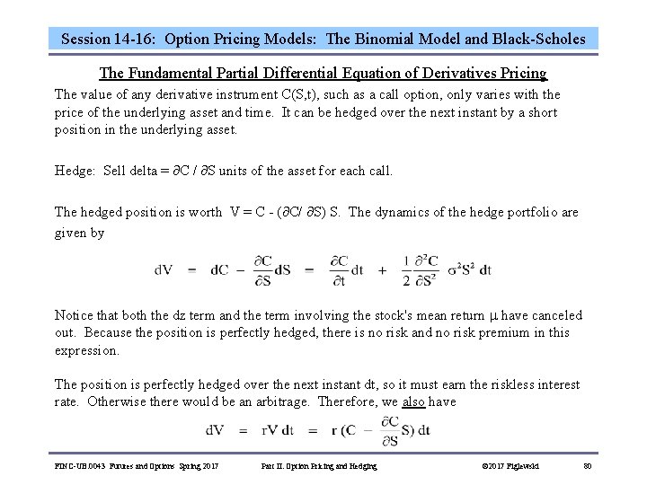
Session 14 -16: Option Pricing Models: The Binomial Model and Black-Scholes The Fundamental Partial Differential Equation of Derivatives Pricing The value of any derivative instrument C(S, t), such as a call option, only varies with the price of the underlying asset and time. It can be hedged over the next instant by a short position in the underlying asset. Hedge: Sell delta = C / S units of the asset for each call. The hedged position is worth V = C - ( C/ S) S. The dynamics of the hedge portfolio are given by Notice that both the dz term and the term involving the stock's mean return have canceled out. Because the position is perfectly hedged, there is no risk and no risk premium in this expression. The position is perfectly hedged over the next instant dt, so it must earn the riskless interest rate. Otherwise there would be an arbitrage. Therefore, we also have FINC-UB. 0043 Futures and Options Spring 2017 Part II: Option Pricing and Hedging © 2017 Figlewski 80

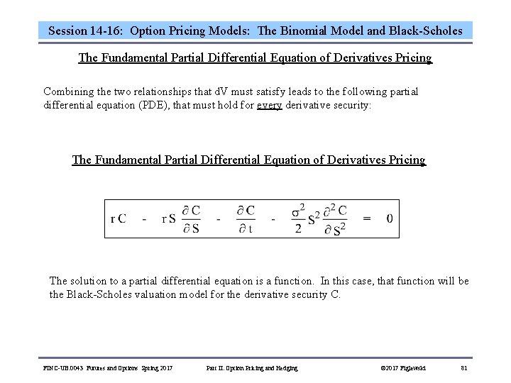
Session 14 -16: Option Pricing Models: The Binomial Model and Black-Scholes The Fundamental Partial Differential Equation of Derivatives Pricing Combining the two relationships that d. V must satisfy leads to the following partial differential equation (PDE), that must hold for every derivative security: The Fundamental Partial Differential Equation of Derivatives Pricing The solution to a partial differential equation is a function. In this case, that function will be the Black-Scholes valuation model for the derivative security C. FINC-UB. 0043 Futures and Options Spring 2017 Part II: Option Pricing and Hedging © 2017 Figlewski 81

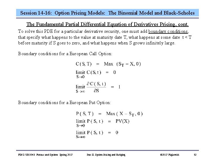
Session 14 -16: Option Pricing Models: The Binomial Model and Black-Scholes The Fundamental Partial Differential Equation of Derivatives Pricing, cont. To solve this PDE for a particular derivative security, one must add boundary conditions, that specify what happens to the value at maturity date T, what happens at some date t < T before maturity if S goes to zero, and what happens when S grows infinitely large. Boundary conditions for a European Call Option: Boundary conditions for a European Put Option: FINC-UB. 0043 Futures and Options Spring 2017 Part II: Option Pricing and Hedging © 2017 Figlewski 82

Session 14 -16: Option Pricing Models: The Binomial Model and Black-Scholes FINC-UB. 0043 Futures and Options Spring 2017 Part II: Option Pricing and Hedging © 2017 Figlewski 83

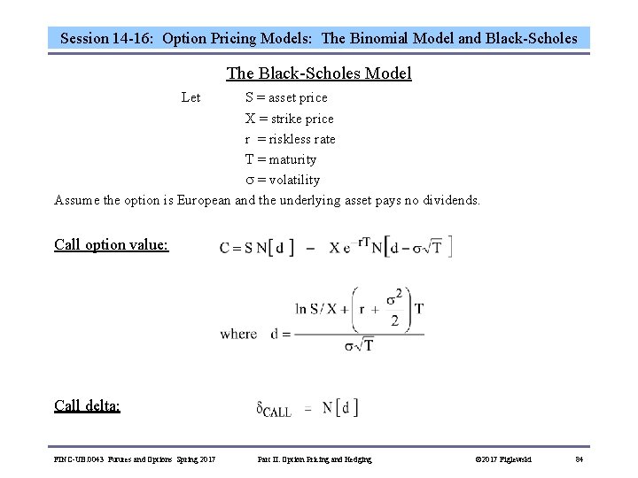
Session 14 -16: Option Pricing Models: The Binomial Model and Black-Scholes The Black-Scholes Model Let S = asset price X = strike price r = riskless rate T = maturity = volatility Assume the option is European and the underlying asset pays no dividends. Call option value: Call delta: FINC-UB. 0043 Futures and Options Spring 2017 Part II: Option Pricing and Hedging © 2017 Figlewski 84

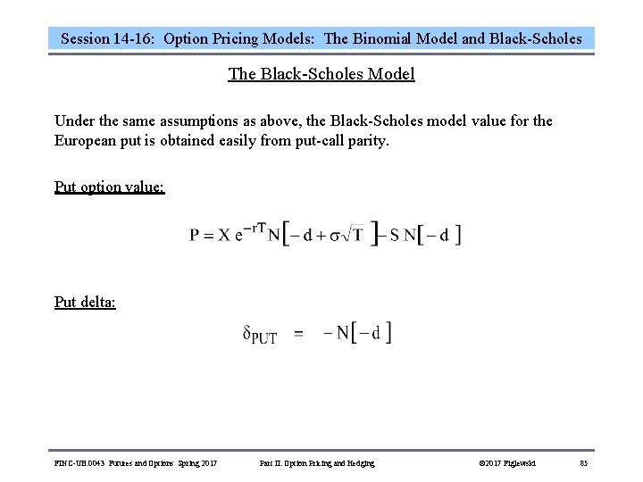
Session 14 -16: Option Pricing Models: The Binomial Model and Black-Scholes The Black-Scholes Model Under the same assumptions as above, the Black-Scholes model value for the European put is obtained easily from put-call parity. Put option value: Put delta: FINC-UB. 0043 Futures and Options Spring 2017 Part II: Option Pricing and Hedging © 2017 Figlewski 85

Session 17: Delta Hedging and Beyond Designing and evaluating option positions requires use of a software implementation of an option pricing model. Rather than use a canned package like the one that comes with the Hull textbook, we have an Excel spreadsheet with the Black-Scholes option pricing model laid out in a few cells. This allows you to develop your own customized analysis tool. [Tricks you can do with the Option Calculator Spreadsheet] FINC-UB. 0043 Futures and Options Spring 2017 Part II: Option Pricing and Hedging © 2017 Figlewski 86

Session 17: Delta Hedging and Beyond The Partial Derivatives of the Call Value Function The partial derivative of the call value with respect to a small change in the stock price is the option's delta. Delta is often written using the Greek letter delta, either (lower case) or (upper case). We will use . Delta serves the same function as the hedge ratio in a futures hedge. It tells how many units of the underlying asset one should trade in order to hedge the market risk exposure of the option. For example, if = 0. 50 for a given call option, the position that is long one call and short 0. 50 shares of stock will be hedged against a (small) change in the stock price up or down. This is called a "delta hedge" and the hedged position is said to be "delta neutral. " FINC-UB. 0043 Futures and Options Spring 2017 Part II: Option Pricing and Hedging © 2017 Figlewski 87

Session 17: Delta Hedging and Beyond The Partial Derivatives of the Call Value Function A very important problem with delta hedging is that delta changes as the stock price moves. The delta of a call option ranges from 0, for an option that is very far out of the money, to 1. 0 for a call that is very deep in the money. Delta hedging requires rebalancing the proportions of stock and the option continuously, as the stock price moves and as time elapses. How much delta changes as S moves is given by the partial derivative of delta with respect to S. This is the second partial derivative of the option value with respect to S. This concept is called by another Greek letter, gamma ( ). Gamma is related to the curvature of the option value function. Positive gamma means the function is convex. The other partial derivatives of the option function are also of importance in hedging, so the Greek alphabet is well represented. These measures of exposure to different types of risk affecting option value are commonly known as "the Greeks. " FINC-UB. 0043 Futures and Options Spring 2017 Part II: Option Pricing and Hedging © 2017 Figlewski 88

Session 17: Delta Hedging and Beyond "Greek Letter" Risk Exposures for Options Delta ( ) - The change in the option value produced by a 1 point change in the price of the underlying asset. Delta measures exposure to Market Risk. Gamma ( ) - The change in the delta produced by a 1 point change in the price of the underlying asset. Gamma measures Convexity, which turns into risk for a delta neutral hedge. Vega - The change in the option value produced by a 1 percentage point change in the volatility of the underlying asset. Vega measures exposure to Volatility Risk (despite not being a true letter in the Greek alphabet). Vega is sometimes written as (which is actually upper case lambda) or as , (which is a Greek nu). Theta ( ) - The change in the option value produced by a 1 day drop in the time to maturity. Theta measures Time Decay. Rho ( ) - The change in the option value produced by a 1 percentage point change in the interest rate. Rho measures exposure to Interest Rate Risk. FINC-UB. 0043 Futures and Options Spring 2017 Part II: Option Pricing and Hedging © 2017 Figlewski 89

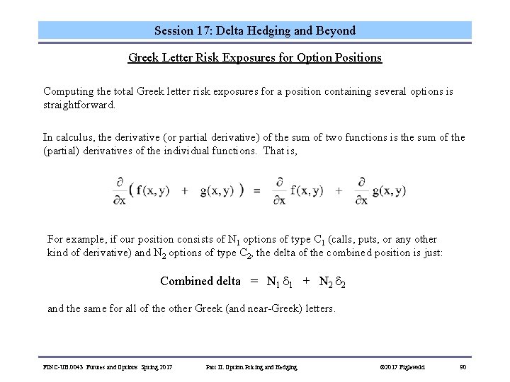
Session 17: Delta Hedging and Beyond Greek Letter Risk Exposures for Option Positions Computing the total Greek letter risk exposures for a position containing several options is straightforward. In calculus, the derivative (or partial derivative) of the sum of two functions is the sum of the (partial) derivatives of the individual functions. That is, For example, if our position consists of N 1 options of type C 1 (calls, puts, or any other kind of derivative) and N 2 options of type C 2, the delta of the combined position is just: Combined delta = N 1 1 + N 2 2 and the same for all of the other Greek (and near-Greek) letters. FINC-UB. 0043 Futures and Options Spring 2017 Part II: Option Pricing and Hedging © 2017 Figlewski 90

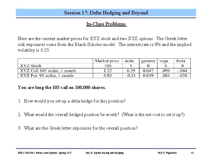
Session 17: Delta Hedging and Beyond In-Class Problems Here are the current market prices for XYZ stock and two XYZ options. The Greek letter risk exposures come from the Black-Scholes model. The interest rate is 8% and the implied volatility is 0. 25. You are long the 105 call on 100, 000 shares. 1. How would you set up a delta hedge for this position? 2. What would the overall hedged position be worth? (What is the net cost to set it up? ) 3. What are the Greek letter exposures for the overall position? FINC-UB. 0043 Futures and Options Spring 2017 Part II: Option Pricing and Hedging © 2017 Figlewski 91

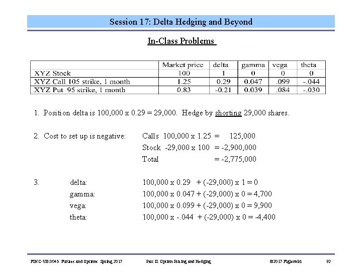
Session 17: Delta Hedging and Beyond In-Class Problems 1. Position delta is 100, 000 x 0. 29 = 29, 000. Hedge by shorting 29, 000 shares. 2. Cost to set up is negative: Calls 100, 000 x 1. 25 = 125, 000 Stock -29, 000 x 100 = -2, 900, 000 Total = -2, 775, 000 3. 100, 000 x 0. 29 + (-29, 000) x 1 = 0 100, 000 x 0. 047 + (-29, 000) x 0 = 4, 700 100, 000 x 0. 099 + (-29, 000) x 0 = 9, 900 100, 000 x -. 044 + (-29, 000) x 0 = -4, 400 delta: gamma: vega: theta: FINC-UB. 0043 Futures and Options Spring 2017 Part II: Option Pricing and Hedging © 2017 Figlewski 92

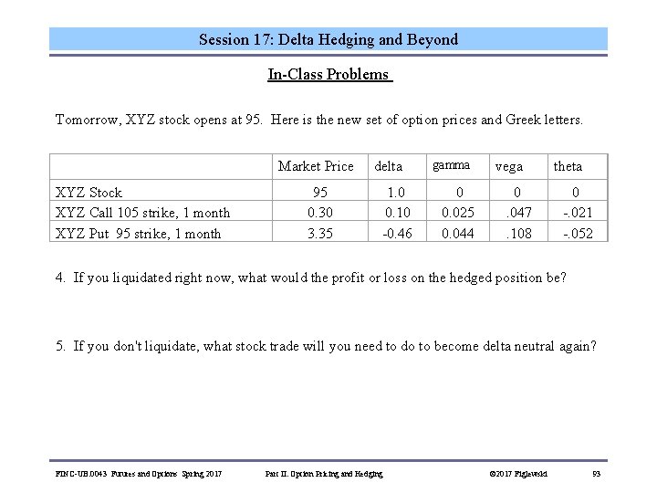
Session 17: Delta Hedging and Beyond In-Class Problems Tomorrow, XYZ stock opens at 95. Here is the new set of option prices and Greek letters. XYZ Stock XYZ Call 105 strike, 1 month XYZ Put 95 strike, 1 month Market Price 95 0. 30 3. 35 delta 1. 0 0. 10 -0. 46 gamma 0 0. 025 0. 044 vega 0 . 047. 108 theta 0 -. 021 -. 052 4. If you liquidated right now, what would the profit or loss on the hedged position be? 5. If you don't liquidate, what stock trade will you need to do to become delta neutral again? FINC-UB. 0043 Futures and Options Spring 2017 Part II: Option Pricing and Hedging © 2017 Figlewski 93

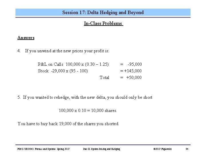
Session 17: Delta Hedging and Beyond In-Class Problems Answers 4. If you unwind at the new prices your profit is: P&L on Calls 100, 000 x (0. 30 – 1. 25) Stock -29, 000 x (95 - 100) Total = -95, 000 = +145, 000 = +50, 000 5. If you wanted to rehedge, with the new delta, you should only be short 100, 000 x 0. 10 = 10, 000 shares. You have to buy back 19, 000 of the shares you shorted. FINC-UB. 0043 Futures and Options Spring 2017 Part II: Option Pricing and Hedging © 2017 Figlewski 94

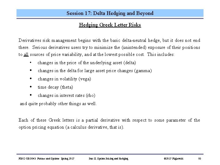
Session 17: Delta Hedging and Beyond Hedging Greek Letter Risks Derivatives risk management begins with the basic delta-neutral hedge, but it does not end there. Serious derivatives users try to minimize the (unintended) exposure of their positions to all sources of price variability, and at the lowest possible cost. This includes: • changes in the price of the underlying asset (delta) • • changes in the delta for large asset price changes (gamma) changes in volatility (vega) time decay (theta) changes in interest rates (rho) and quite probably other things as well. Each of these Greek letters is a partial derivative with respect to some parameter of the option pricing equation (a calculus derivative, that is). FINC-UB. 0043 Futures and Options Spring 2017 Part II: Option Pricing and Hedging © 2017 Figlewski 95

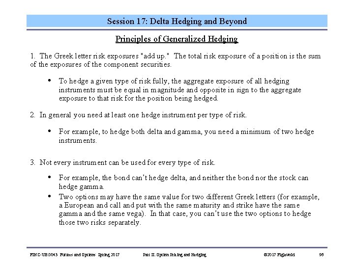
Session 17: Delta Hedging and Beyond Principles of Generalized Hedging 1. The Greek letter risk exposures "add up. " The total risk exposure of a position is the sum of the exposures of the component securities. • To hedge a given type of risk fully, the aggregate exposure of all hedging instruments must be equal in magnitude and opposite in sign to the aggregate exposure to that risk for the position being hedged. 2. In general you need at least one hedge instrument per type of risk. • For example, to hedge both delta and gamma, you need a minimum of two hedge instruments. 3. Not every instrument can be used for every type of risk. • • For example, the bond can’t hedge delta, and neither the bond nor the stock can hedge gamma. Two options may have the same value for two different Greek letters (for example, a European and call and put with the same maturity and strike have the same gamma and the same vega). In that case, you can’t use the two options to hedge those two risks separately. FINC-UB. 0043 Futures and Options Spring 2017 Part II: Option Pricing and Hedging © 2017 Figlewski 96

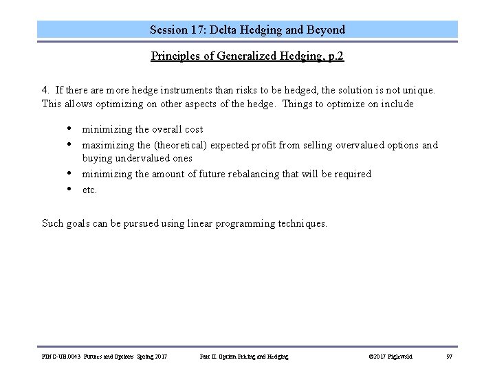
Session 17: Delta Hedging and Beyond Principles of Generalized Hedging, p. 2 4. If there are more hedge instruments than risks to be hedged, the solution is not unique. This allows optimizing on other aspects of the hedge. Things to optimize on include • • minimizing the overall cost maximizing the (theoretical) expected profit from selling overvalued options and buying undervalued ones minimizing the amount of future rebalancing that will be required etc. Such goals can be pursued using linear programming techniques. FINC-UB. 0043 Futures and Options Spring 2017 Part II: Option Pricing and Hedging © 2017 Figlewski 97

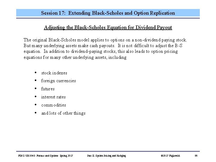
Session 17: Extending Black-Scholes and Option Replication Adjusting the Black-Scholes Equation for Dividend Payout The original Black-Scholes model applies to options on a non-dividend paying stock. But many underlying assets make cash payouts. It is not difficult to adjust the B-S equation. In addition to dividend-paying stocks, this also leads to option pricing equations for many other underlying assets, including • • • stock indexes foreign currencies futures interest rates commodities and lots of other things FINC-UB. 0043 Futures and Options Spring 2017 Part II: Option Pricing and Hedging © 2017 Figlewski 98

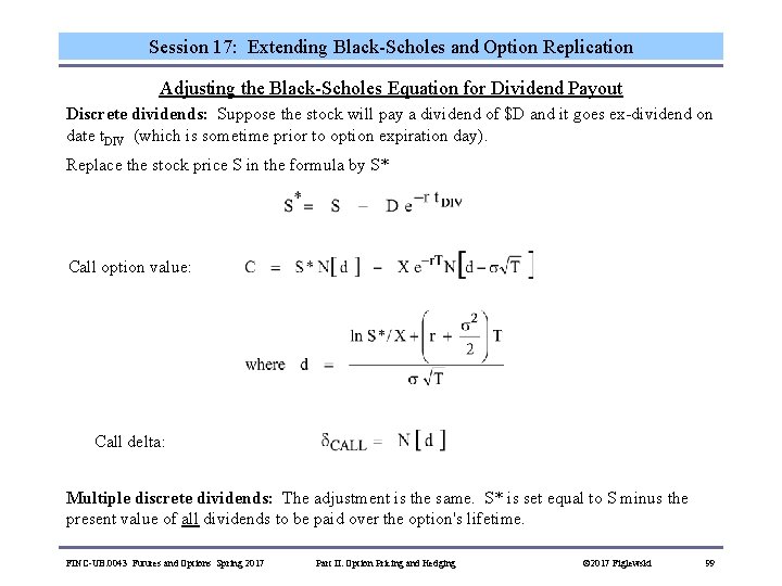
Session 17: Extending Black-Scholes and Option Replication Adjusting the Black-Scholes Equation for Dividend Payout Discrete dividends: Suppose the stock will pay a dividend of $D and it goes ex-dividend on date t. DIV (which is sometime prior to option expiration day). Replace the stock price S in the formula by S* Call option value: Call delta: Multiple discrete dividends: The adjustment is the same. S* is set equal to S minus the present value of all dividends to be paid over the option's lifetime. FINC-UB. 0043 Futures and Options Spring 2017 Part II: Option Pricing and Hedging © 2017 Figlewski 99

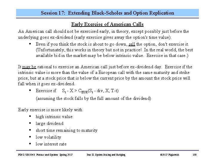
Session 17: Extending Black-Scholes and Option Replication Early Exercise of American Calls An American call should not be exercised early, in theory, except possibly just before the underlying goes ex-dividend (early exercise gives away the option's time value). • Even if you think the stock is about to go down, sell the option, don't exercise it. (Unfortunately, this works in theory but not in practice! In the real world, the best available bid in the market may be below intrinsic value. Exercise in that case. ) It may be rational to exercise an American call just before ex-dividend day. Exercise if the intrinsic value is more than the value of a European call with the same maturity and strike price, but at a stock price that is below the current price by the amount the stock price will fall when it goes ex-dividend. • Exercise if St - X > CEUR(St - div, X, T-t) (assuming the stock falls by the full amount of the dividend) Early exercise is more likely with • high intrinsic value • large dividend • short time remaining to maturity • low volatility • low interest rate FINC-UB. 0043 Futures and Options Spring 2017 Part II: Option Pricing and Hedging © 2017 Figlewski 100

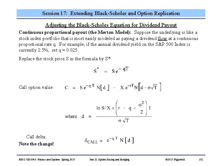
Session 17: Extending Black-Scholes and Option Replication Adjusting the Black-Scholes Equation for Dividend Payout Continuous proportional payout (the Merton Model): Suppose the underlying is like a stock index portfolio that is most easily modeled as paying a dividend flow at a continuous proportional rate q. For example, if the annual dividend yield on the S&P 500 Index is currently 2. 5%, set q = 0. 025. Replace the stock price S in the formula by S*: Call option value: Call delta: Note the change! FINC-UB. 0043 Futures and Options Spring 2017 Part II: Option Pricing and Hedging © 2017 Figlewski 101

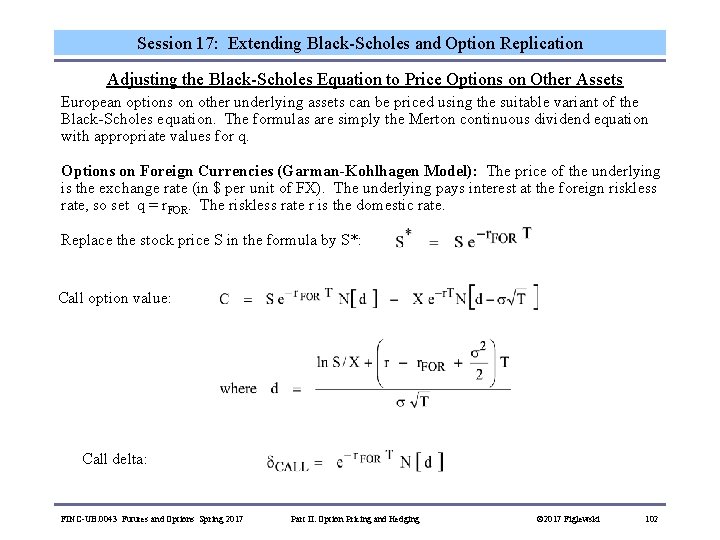
Session 17: Extending Black-Scholes and Option Replication Adjusting the Black-Scholes Equation to Price Options on Other Assets European options on other underlying assets can be priced using the suitable variant of the Black-Scholes equation. The formulas are simply the Merton continuous dividend equation with appropriate values for q. Options on Foreign Currencies (Garman-Kohlhagen Model): The price of the underlying is the exchange rate (in $ per unit of FX). The underlying pays interest at the foreign riskless rate, so set q = r. FOR. The riskless rate r is the domestic rate. Replace the stock price S in the formula by S*: Call option value: Call delta: FINC-UB. 0043 Futures and Options Spring 2017 Part II: Option Pricing and Hedging © 2017 Figlewski 102

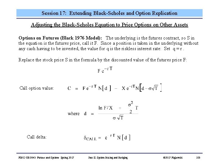
Session 17: Extending Black-Scholes and Option Replication Adjusting the Black-Scholes Equation to Price Options on Other Assets Options on Futures (Black 1976 Model): The underlying is the futures contract, so S in the equation is the futures price, call it F. Since a position is taken in the underlying without any cash having to be invested, the value for q is the riskless interest rate: Set q = r. Replace the stock price S in the formula by the discounted value of the futures price F: Call option value: Call delta: FINC-UB. 0043 Futures and Options Spring 2017 Part II: Option Pricing and Hedging © 2017 Figlewski 103

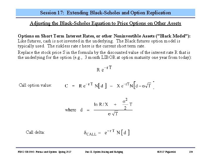
Session 17: Extending Black-Scholes and Option Replication Adjusting the Black-Scholes Equation to Price Options on Other Assets Options on Short Term Interest Rates, or other Noninvestible Assets ("Black Model"): Like futures, cash is not invested in the underlying. The Black futures option model is typically used. The riskless rate r here is the current short term rate. Replace the stock price S in the formula by the discounted value of the interest rate R that is the underlying for the option (e. g. , 3 month LIBOR at option maturity one year from today): Call option value: Call delta: FINC-UB. 0043 Futures and Options Spring 2017 Part II: Option Pricing and Hedging © 2017 Figlewski 104

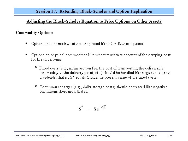
Session 17: Extending Black-Scholes and Option Replication Adjusting the Black-Scholes Equation to Price Options on Other Assets Commodity Options: • Options on commodity futures are priced like other futures options. • Options on physical commodities like wheat must take account of the carrying costs for the underlying. ° Fixed costs (e. g. , an inspection fee, the cost of transporting the deliverable commodity to the delivery point, etc. ) should be handled like negative discrete dividends, that is, S* equals S plus the present value of the fixed costs. ° Continuous charges (e. g. , daily storage costs) should be treated like negative continuous dividends, that is, FINC-UB. 0043 Futures and Options Spring 2017 Part II: Option Pricing and Hedging © 2017 Figlewski 105

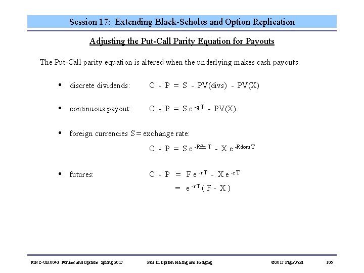
Session 17: Extending Black-Scholes and Option Replication Adjusting the Put-Call Parity Equation for Payouts The Put-Call parity equation is altered when the underlying makes cash payouts. • discrete dividends: C - P = S - PV(divs) - PV(X) • continuous payout: C - P = S e -q T - PV(X) • foreign currencies S = exchange rate: C - P = S e -Rfor T - X e -Rdom T • futures: C - P = F e -r T - X e -r T = e -r T ( F - X ) FINC-UB. 0043 Futures and Options Spring 2017 Part II: Option Pricing and Hedging © 2017 Figlewski 106

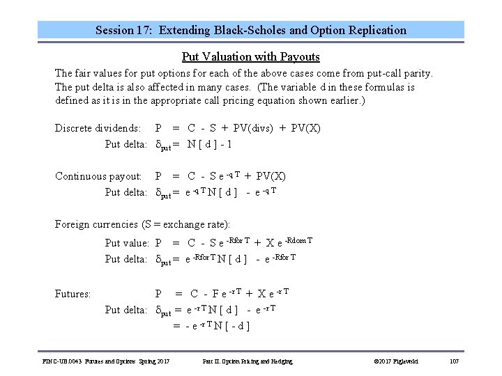
Session 17: Extending Black-Scholes and Option Replication Put Valuation with Payouts The fair values for put options for each of the above cases come from put-call parity. The put delta is also affected in many cases. (The variable d in these formulas is defined as it is in the appropriate call pricing equation shown earlier. ) Discrete dividends: P = C - S + PV(divs) + PV(X) Put delta: put = N [ d ] - 1 Continuous payout: P = C - S e -q T + PV(X) Put delta: put = e -q T N [ d ] - e -q T Foreign currencies (S = exchange rate): Put value: P = C - S e -Rfor T + X e -Rdom T Put delta: put = e -Rfor T N [ d ] - e -Rfor T Futures: P = C - F e -r T + X e -r T Put delta: put = e -r T N [ d ] - e -r T = - e -r T N [ - d ] FINC-UB. 0043 Futures and Options Spring 2017 Part II: Option Pricing and Hedging © 2017 Figlewski 107

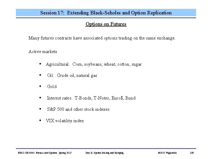
Session 17: Extending Black-Scholes and Option Replication Options on Futures Many futures contracts have associated options trading on the same exchange. Active markets • Agricultural: Corn, soybeans, wheat, cotton, sugar • Oil: Crude oil, natural gas • Gold • Interest rates: T-Bonds, T-Notes, Euro$, Bund • S&P 500 and other stock indexes • VIX volatility index FINC-UB. 0043 Futures and Options Spring 2017 Part II: Option Pricing and Hedging © 2017 Figlewski 108

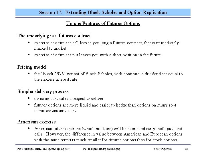
Session 17: Extending Black-Scholes and Option Replication Unique Features of Futures Options The underlying is a futures contract • • exercise of a futures call leaves you long a futures contract, that is immediately marked to market exercise of a futures put leaves you with a short position in the future Pricing model • the "Black 1976" variant of Black-Scholes, with continuous dividend set equal to the riskless interest rate Simpler delivery process • • no issue of what is cheapest to deliver futures options are more liquid and easier to hedge than options on many spot commodities and assets American exercise • American futures options (which most are) will be exercised early, both puts and calls. However, the difference in value between American and European options with the same terms is much smaller for futures options than for stock options. FINC-UB. 0043 Futures and Options Spring 2017 Part II: Option Pricing and Hedging © 2017 Figlewski 109

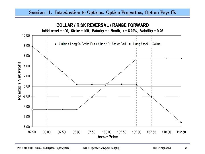
Session 17: Extending Black-Scholes and Option Replication Unique Features of OTC Foreign Currency Options Price quotes are in terms of "vols, " i. e. , the volatility parameter to be input into the Garman. Kohlhagen pricing equation. "Moneyness, " if expressed in dollar terms, is quoted relative to the forward rate. • For example, if the spot rate on the Euro is 1. 35 and the three month forward is 1. 36, a three month "at the money forward" (ATMF) call will be struck at 1. 36. Usually, though, an option's moneyness is defined in terms of its delta. • A "25 -delta" call, will be one whose delta according to the formula is 0. 25. A 25 delta put has delta of -0. 25. Quotes (in vol terms) are often given on combination positions: • Straddle: Long a call and a put with the same maturity, both struck at the money forward. • Strangle: Long a 25 -delta call and a 25 -delta put (i. e. , both are out of the money). • Risk Reversal: Long a 25 -delta put, short a 25 -delta call (also called a "Range Forward" or a "Collar"). FINC-UB. 0043 Futures and Options Spring 2017 Part II: Option Pricing and Hedging © 2017 Figlewski 110

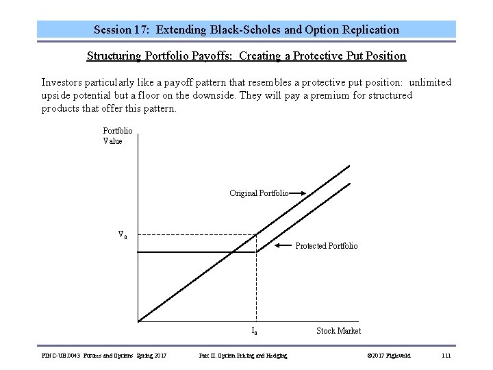
Session 17: Extending Black-Scholes and Option Replication Structuring Portfolio Payoffs: Creating a Protective Put Position Investors particularly like a payoff pattern that resembles a protective put position: unlimited upside potential but a floor on the downside. They will pay a premium for structured products that offer this pattern. Portfolio Value Original Portfolio V 0 Protected Portfolio I 0 Stock Market FINC-UB. 0043 Futures and Options Spring 2017 Part II: Option Pricing and Hedging © 2017 Figlewski 111

Session 17: Extending Black-Scholes and Option Replication Buying Put Protection with Options on a Specific Portfolio Securities firms will create and sell options that their customers want to buy, including a put option on a specific portfolio. Consider buying a protective put on a portfolio that is currently worth V 0 = $100 million. The objective is to place a floor of $96 million on the total portfolio value in 1 year. The parameters of the problem are: V 0 = 100 Floor = 96 Horizon = 1 year Riskless interest = 8. 00% Portfolio volatility = 0. 20 No dividends (dividends to be received are simply included in the value of the portfolio to be guaranteed) There are several different ways to set the problem up. It is important to distinguish clearly between changes in the amount of stock in the portfolio from purchases and sales, versus changes in the prices of the stocks. We only want to be protected against price changes. FINC-UB. 0043 Futures and Options Spring 2017 Part II: Option Pricing and Hedging © 2017 Figlewski 112

Session 17: Extending Black-Scholes and Option Replication Buying Put Protection with Options on a Specific Portfolio, p. 2 The underlying asset for the put option is the whole portfolio, whose value V is assumed to follow the standard Black-Scholes lognormal diffusion. That is, one put is based on one "share" of portfolio, whose price is the portfolio's current market value. Setting the asset value V 0 = 100, and the put strike price equal to the desired floor, X = Floor = 96, the Black-Scholes value for the put is P(V 0, X) = P(100, 96) = $3. 230 million Buying this put would guarantee that if the value of our $100 million portfolio is below $96 million a year from now, the protective put will make up the difference. A problem with this solution is that it costs more than we have to invest: Cost = V 0 + P(V 0, X) = 100 + 3. 230 = 103. 230. If we sell off some stock to buy the put, we don't have $100 million invested anymore. A 96 strike put is not so far out of the money relative to our new smaller portfolio, so it will cost more than what we just calculated. It is not hard to find the solution to this problem by iteration. We will find that if $100 million is all we can invest, the protective put that gives a floor of 96 will cost $4. 506 million and we will only have $95. 494 left to invest in stocks. FINC-UB. 0043 Futures and Options Spring 2017 Part II: Option Pricing and Hedging © 2017 Figlewski 113

Session 17: Extending Black-Scholes and Option Replication Creating the Protective Put Payoff Synthetically with a "Portfolio Insurance" Strategy A big problem with buying a put on a specific portfolio is that such options are not widely traded. We have to find a securities firm willing to write the puts, and then negotiate an acceptable price. (This used to be a bigger problem than it is today. ) In the late 1970 s, two Berkeley finance professors, Hayne Leland Mark Rubinstein, proposed, and began marketing, an idea they called "Portfolio Insurance. " It amounted to a dynamic trading strategy that would replicate the desired protective put payoff, simply by trading between the original portfolio and riskless bonds. The concept is simple. The basic replicating strategy for any option position is simply to hold an amount of the underlying that will have the same delta as the desired position and to borrow or lend enough of the riskless asset so that the total replicating portfolio has the same cost. THIS IS A KEY POINT TO REMEMBER! Important: The following two steps give the general procedure to replicate an option: 1. Use the underlying (or some other derivative tied to the underlying, such as a futures contract) to produce the same delta as the option one is trying to replicate. 2. Use riskless borrowing or lending to make the cost of the replicating position equal to theoretical price of the option. FINC-UB. 0043 Futures and Options Spring 2017 Part II: Option Pricing and Hedging © 2017 Figlewski 114

Session 17: Extending Black-Scholes and Option Replication Creating the Protective Put Payoff Synthetically using "Portfolio Insurance" We have calculated that for our example, the amount of stock to keep, Vp, is Vp = V 0 - P(Vp, X) = 100 - 4. 506 = 95. 494 million For the purpose of calculating a delta, we treat our stock position Vp as being one "share" of portfolio with a current price of $95. 494 million. • Using the Black-Scholes model, with S = 95. 494, the put's delta is -0. 3233. • Just as if it were 1 share of stock, the delta of Vp is 1. 0. FINC-UB. 0043 Futures and Options Spring 2017 Part II: Option Pricing and Hedging © 2017 Figlewski 115

Session 17: Extending Black-Scholes and Option Replication Creating the Protective Put Payoff Synthetically using "Portfolio Insurance, " p. 2 The replicating portfolio for the put alone is • • • short 0. 3233 units of Vp: -0. 3233 x 95. 494 = -$30. 873 million of Vp lend at the riskless rate to make the total out of pocket cost = the price of the put we are trying to replicate, which is 4. 506: ==> lend 4. 506 + 30. 873 = $35. 379 million. The overall portfolio insurance protected portfolio is therefore: • • $95. 494 - $30. 873 = $64. 621 million of Vp (sell off $35. 379 million of the original stocks) $35. 379 million in riskless bonds This position will have to be rebalanced regularly to maintain the right delta as stock prices change. This may be hard to do. It requires selling stocks to reduce effective market exposure when stock prices are falling, and buying stocks when prices are rising. (Ask about what happened on October 19, 1987. ) FINC-UB. 0043 Futures and Options Spring 2017 Part II: Option Pricing and Hedging © 2017 Figlewski 116

Session 17: Extending Black-Scholes and Option Replication A Hybrid Security for Retail Investors: The Equity-Linked CD An equity-linked CD is a type of certificate of deposit, whose payoff is tied to the stock market, but with downside protection of principal. Typical structure: The deposit has a maturity of five years, during which time it pays no interest. At maturity, the initial deposit is returned, plus interest equal to the percentage increase in the level of the S&P 500 stock index over the five years. If the S&P goes down, the initial principal is returned in full but there is no additional interest payment. FINC-UB. 0043 Futures and Options Spring 2017 Part II: Option Pricing and Hedging © 2017 Figlewski 117

Session 17: Extending Black-Scholes and Option Replication Designing an Equity-Linked CD Suppose you have the following data: S&P index S&P dividend yield S&P volatility Issuing bank's normal interest rate on a 5 year zero coupon CD 1000 2. 9%. 137 5. 30% 1) Per $100 invested, what does it cost the bank in present value terms to provide this payoff structure? FINC-UB. 0043 Futures and Options Spring 2017 Part II: Option Pricing and Hedging © 2017 Figlewski 118

Session 17: Extending Black-Scholes and Option Replication Designing an Equity-Linked CD To get downside protection of principal, buy a five year zero coupon bond with 100 face value. At 5. 30 percent interest, 5 -year zero, $100 face value = 100 / (1. 0530)5 = 77. 24 To get the upside price appreciation on the S&P, buy a 5 -year call option. • The underlying is $100 worth of the S&P portfolio. As before, think of this as "one unit of an underlying asset whose current price is 100. " • The call should be at-the-money, so set the strike to 100. (Note: Because we are doing everything in terms of rates of return, the current level of the S&P is not used in solving this problem. ) 5 -year at the money call on $100 of the S&P 500 = 15. 39 This leaves an immediate profit to the bank: Profit = Deposit - bond price - call price = 100 – 77. 24 – 15. 39 = 7. 36 FINC-UB. 0043 Futures and Options Spring 2017 Part II: Option Pricing and Hedging © 2017 Figlewski 119

Session 17: Extending Black-Scholes and Option Replication Designing an Equity-Linked CD $7. 36 per $100 deposited is a high profit rate. Competition will surely drive it down. Suppose the bank limits fee to 2 percent of principal, taken out at the beginning. The remainder of the deposit is then used to lock in the minimum payment at maturity and to provide equity market exposure. One alternative would be for the account to pay a small interest rate on the deposit, in addition to 100 percent of the appreciation of the stock index. Alternative #1: Full matching of the S&P on the upside plus payment of a fixed interest rate if the S&P falls. Deposit 100 less cost of call option -15. 39 less bank profit - 2 equals amount available to buy zeros = 82. 61 Buying $82. 61 of 5 -year zeros produces 82. 61 x 1. 05305 = $106. 94 at maturity. This corresponds to: annual interest rate = 1. 35% FINC-UB. 0043 Futures and Options Spring 2017 Part II: Option Pricing and Hedging © 2017 Figlewski 120

Session 17: Extending Black-Scholes and Option Replication Designing an Equity-Linked CD Alternatively, the bank can limit its fee to 2 percent of principal and use the extra funds to give greater than 100 percent of the appreciation on the index, if it goes up. Alternative #2: Guaranteed return of principal without interest if the market goes down, and more than 100% of the S&P capital gain if it goes up. Deposit 100 less cost of 5 -year zeros -77. 24 less bank profit - 2 equals amount available to buy calls = 20. 76 By buying calls on more than $100 worth of the S&P 500, the bank can guarantee return of $100 principal plus 20. 76 / 15. 39 = 134% of the S&P capital gain. FINC-UB. 0043 Futures and Options Spring 2017 Part II: Option Pricing and Hedging © 2017 Figlewski 121

Session 18: Volatility Modern option pricing models following Black-Scholes all have a major role for the volatility of the underlying asset's return. This is the one parameter in Black-Scholes that is not observable, so naturally there is a lot of dispersion around the average volatility expectation in the market. In Black-Scholes, volatility is assumed to be a constant known parameter. But in the real world it is neither constant nor known. This session will review what we know about volatility, how it goes into option prices, and how the wide variety of volatility-based products can be used to speculate or hedge volatility. FINC-UB. 0043 Futures and Options Spring 2017 Part II: Option Pricing and Hedging © 2017 Figlewski 122

Volatility: Flowchart of How Volatility Gets into Option Prices and How it is Extracted Historical price data Forecasts and other information Hedging (risk aversion) Statistical Estimate of Future Returns Investors' Estimate of Future Returns Demand for Options Market Option Prices Invert the Black. Scholes Model Implied BS Volatilities Volatility smile What a financial econometrician calculates What the market actually predicts: the "P" density also known as "empirical" or "real world" probabilities What the options market embeds in option prices, including risk premia: the "Q" density, Model-free Volatility calculation "Risk-neutral" Probabilities Volatility surface Risk Neutral Density The original VIX Index VXO Model-free Implied Volatility; the VIX Index

Session 18: Volatility "Stylized Facts" about Volatility Here are some common findings from research on the behavior of asset volatility • • • volatility is not constant; it changes substantially over time • in equity markets, volatility increases when stock prices fall, and (may) decrease when prices rise (this is often called the "leverage effect") • implied volatility has a regular structure across options with different strike prices, known as the "smile" or the "skew" • implied volatility also shows systematic "term structure" effects for options with different maturities periods of high volatility and periods of low volatility cluster togethere appears to be "mean reversion" in volatility; periods of unusually high or low volatility tend to be followed by a reversion to more normal behavior FINC-UB. 0043 Futures and Options Spring 2017 Part II: Option Pricing and Hedging © 2017 Figlewski 124

Session 18: Volatility Three Techniques for Estimating / Forecasting Volatility from Historical Data 1. Historical volatility: • Compute K log returns from past prices: Rt-k = ln( St-k / St-k-1 ), for k = 1, . . . , K • Volatility estimate = annualized standard deviation of {R} FINC-UB. 0043 Futures and Options Spring 2017 Part II: Option Pricing and Hedging © 2017 Figlewski 125

Session 18: Volatility Three Techniques for Estimating / Forecasting Volatility from Historical Data 2. Exponentially weighted moving average • • Compute log returns from past data as above Downweight data as it ages, by multiplying each squared deviation by wk, for some weight w < 1. 0. (Riskmetrics uses w = 0. 94. ) • Volatility estimate = annualized value of FINC-UB. 0043 Futures and Options Spring 2017 Part II: Option Pricing and Hedging © 2017 Figlewski 126

Session 18: Volatility 3. GARCH (Generalized Autoregressive Conditional Heteroskedasticity) Model variance at date t as a combination of � last period's variance, 2 t-1 � last period's squared random price shock 2 t-1 The simplest GARCH model has two equations: Return equation: rt = µ + t , t is distributed as Normal (0, 2 t) Variance equation: 2 t = C + a 2 t-1 + b 2 t-1 (Typical values are 0. 90 to 0. 95 for a and 0. 05 to 0. 08 for b. The sum should be < 1. 0. ) For stocks an asymmetry term is added to make volatility go up when the stock price falls. The GARCH model for stock returns: 2 t = C + a 2 t-1 + b 2 t-1 + d 2 t-1 (if t-1 < 0) Note that in the GARCH framework, time is not continuous. FINC-UB. 0043 Futures and Options Spring 2017 Part II: Option Pricing and Hedging © 2017 Figlewski 127

Session 18: Volatility Practical Issues in Estimating Volatility from Past Prices If the price of the underlying asset did follow a lognormal diffusion with constant mean and volatility, as assumed by Black and Scholes, you would get the best volatility estimate by using as much past data, sampled at as fine an interval, as you could get. But with real world prices, several practical issues arise: • what observation interval to use (daily? monthly? intraday? ) • suggestion: higher frequency is better, so use daily data; intraday returns require special handling • whether to estimate the mean • NO! • how much past data to include • as much as possible, but not from much different economic environments • how to deal with "outliers, " i. e. , events like October 19, 1987 • there is no perfect answer; use judgment and consider how sensitive the results are to the outliers FINC-UB. 0043 Futures and Options Spring 2017 Part II: Option Pricing and Hedging © 2017 Figlewski 128

Session 18: Volatility Conclusions on Forecasting Volatility: Historical Data Here are several general conclusions I have reached based on my research on volatility prediction • • Different methods should be compared in terms of out of sample forecasting performance Accuracy of all methods is low Using data sampled at very short intervals (daily or less) requires careful adjustment for "noise" arising from the trading process (e. g. , "bid-ask bounce") It is better to assume the mean is 0 than to take deviations around the sample mean. Simpler models, such as straightforward use of measured historical volatility over a long sample period seem to be about as accurate as more complicated models, and are more robust. Volatility forecasts for long horizons seem to be more accurate than for short horizons GARCH models appear to work well over very short horizons, but only if there is a lot of data available to estimate model parameters GARCH seems to work best for equities. FINC-UB. 0043 Futures and Options Spring 2017 Part II: Option Pricing and Hedging © 2017 Figlewski 129

Session 18: Volatility Implied volatility is the value of the volatility input to an option pricing model that makes the model value equal the option price observed in the market. IV is the solution to C(S, X, T, r, IV) = Cmarket (The actual value for IV must be found by a search process. ) IV should impound "the market's" forecast of volatility. IV is felt by many to be the best volatility estimate possible, because the market has access to much more information than any model can incorporate. There is a one-to-one correspondence between implied volatility and option price. In some markets, options are quoted in terms of implied volatility, rather than price. OTC foreign currency options are an important example. Note that implied volatility depends on the option pricing model used to calculate it. IV as commonly reported is always computed from the Black-Scholes model (with dividend correction, and sometimes with an adjustment for American exercise). FINC-UB. 0043 Futures and Options Spring 2017 Part II: Option Pricing and Hedging © 2017 Figlewski 130

Session 18: Volatility The VIX Volatility Index The CBOE computes, publishes, and now trades futures and options based on a composite index known as the VIX. The VIX index is designed to measure the standard deviation of the S&P 500 stock index over the next month, as implied by the current market prices of SPX index options. The index is an interpolated value for a one month horizon, extracted from the nearest to expiration and the next nearest contracts. The original formula for computing the VIX was changed in 2003. The "Old VIX, " (still computed and published as the VXO), was based on 8 at-the-money calls and puts on the OEX index and used the Black-Scholes model to extract the implied volatilities. These IVs were combined into a weighted average 30 -day at-the-money implied volatility. (There was also a technical problem in annualizing the index, which made it significantly biased upward. ) The new VIX uses all out of the money SPX index calls and puts expiring just before and just after 30 days and extracts, not individual IVs, but the whole risk neutral probability distribution (without using Black-Scholes or any other pricing model). The implied volatility is the standard deviation from this implied distribution. Futures contracts on the VIX began trading in 2004 and VIX options in 2006. Although it is supposed to be an estimate of volatility, the VIX is widely thought of and referred to, as "the market fear gauge". FINC-UB. 0043 Futures and Options Spring 2017 Part II: Option Pricing and Hedging © 2017 Figlewski 131

2500 90 Historical and Implied Volatility for S&P 500 Index 80 2000 70 1500 50 40 1000 30 20 500 10 SPX VIX Historical Volatility (last 6 months) 0 0 9/4/1990 5/31/1993 2/25/1996 11/21/1998 8/17/2001 5/13/2004 2/7/2007 11/3/2009 7/30/2012 4/26/2015 132 Volatility S&P 500 Index 60

Vega in Action Implied volatility July 31 Closing price August 1 Closing price Implied volatility August 1

The Volatility Surface

Session 18: Volatility The Real Mystery: Where Does the Volatility Smile Come From? A Variety of Possible Explanations: 1. The underlying returns distribution is not Normal. ("Fat tailed" distributions) • too many "big" returns (both positive and negative); a Student-t distribution with about 7 degrees of freedom fits the data better 2. Volatility of a stock depends on the ratio of equity to debt in the firm's capital structure, and that changes when the stock price moves. (The "leverage effect") 3. Volatility is stochastic • GARCH (volatility is a function of the asset price change) • Two-factor models (in which volatility is subject to random changes that are at least partly independent of the price change) 4. Stock prices can make large jumps (non lognormal "jump-diffusion processes") 5. Investors are "Crash-o-phobic" and are willing to pay extra for the protection of out of the money puts. In the money calls (that have strike prices below the current stock price, like out of the money puts) must also have high implied volatilities or else they would violate put -call parity. FINC-UB. 0043 Futures and Options Spring 2017 Part II: Option Pricing and Hedging © 2017 Figlewski 135

Session 18: Volatility Trading Volatility: Variance Swaps and Vol Swaps There are now multiple ways to trade volatility as an investible asset. The easiest is a variance swap. This is a forward contract on the difference between the realized variance of returns over some period ending at a future date and a strike level set at the beginning. Example: A trader who expects high volatility in the stock market until the end of the year 2016 could "buy" a variance swap with a strike variance rate of (0. 20)2 and maturity Dec. 31. The quote is often done in terms of the volatility implied by the given variance, which is 20% in this case. Realized variance is calculated as the annualized mean of Rt 2 , where Rt is the log return, for dates t from now through Dec. 31. The difference between realized variance and the strike is multiplied by a notional principal to get the payoff in dollars. A volatility swap is essentially the same thing, except the payoff is in terms of the difference between realized volatility and the strike. A volatility swap seems to make more sense, since volatility is what investors care about, but valuation is trickier mathematically, meaning it is a lot harder to hedge than a variance swap, so vol swaps are less popular. FINC-UB. 0043 Futures and Options Spring 2017 Part II: Option Pricing and Hedging © 2017 Figlewski 136

Session 18: Volatility Trading Volatility: Derivatives Based on the VIX In 2004, the CBOE introduced trading in futures contracts based on the VIX. Contract size is $1000 times the VIX index, with minimum tick size of 0. 01 (1 volatility basis point). There is no cost of carry pricing model for VIX products, since you can't store the VIX. In 2006, the CBOE added VIX options, i. e. , options whose payoffs are equal to $100 * Max(VIXT – X, 0), where T is option maturity and X is the strike level. Volatility products have become immensely popular. There are now dozens of related volatility contracts for different commodities and time horizons. There also numerous exchange traded funds that offer exposure to volatility (of stocks, or oil, or gold, or. . . ) just like a mutual fund. These trade like stocks, not futures or options. But they all use VIX futures to create their payoffs. FINC-UB. 0043 Futures and Options Spring 2017 Part II: Option Pricing and Hedging © 2017 Figlewski 137

Session 18: Volatility Trading the VIX and financial products based on the VIX is very different from trading stocks or commodities, because the VIX itself cannot be bought and held. It is not investible. Exchange-traded VIX-based products like ETFs are all based on VIX futures. Gold futures are tied to the current price of gold, because you can buy gold today, hedge by selling futures, and lock in the return on the trade. Similarly, you can buy a portfolio of stocks, sell short index futures, and carry that hedged position to futures maturity. By contrast, the VIX is more like a temperature. The current level can be observed all the time, but you can't buy the VIX, carry it over time and deliver it against a future or option contract. This means: 1. The VIX future is based on expectations about what the VIX will be at futures maturity. There is no arbitrage-based pricing model for the VIX. 2. There is therefore no direct connection between what the spot VIX does and how any VIX products behave, just as today's temperature tells us little about what the temperature will be 30 days from now. FINC-UB. 0043 Futures and Options Spring 2017 Part II: Option Pricing and Hedging © 2017 Figlewski 138

Session 18: Volatility The Information Content of Implied Volatility Question: Is implied volatility from an option's market price an efficient forecast of future volatility of the underlying asset? • Is IV an unbiased forecast? • Does IV impound all of the information contained in historical volatility? This issue has been examined many times in the literature for different markets. Most researchers find IV biased, but that it contains information, and generally more than historical volatility. FINC-UB. 0043 Futures and Options Spring 2017 Part II: Option Pricing and Hedging © 2017 Figlewski 139

Session 18: Volatility The Information Content of Implied Volatility The idea that implied volatility is an efficient forecast of future realized volatility involves a joint hypothesis. 1. The implied volatility IV reveals the market's volatility forecast: IV = EMKT[ ] 2. The market's forecast is rational = EMKT[ ] + where has mean 0 and minimum variance given the currently available information. FINC-UB. 0043 Futures and Options Spring 2017 Part II: Option Pricing and Hedging © 2017 Figlewski 140

Session 18: Volatility The Information Content of Implied Volatility: Standard tests 1. "Rationality test regression: " If F is a rational forecast of volatility , then = F + To test this, run the regression Test = 0 and = 1. 0 t = + Ft + ut 2. "Encompassing regression: " With multiple forecasts F 1 and F 2, run this regression t = + 1 F 1 t + 2 F 2 t + ut; If the F 1 t forecast impounds all of the information contained in F 2 t, then = 0. 0, 1 = 1. 0, and 2 = 0 FINC-UB. 0043 Futures and Options Spring 2017 Part II: Option Pricing and Hedging © 2017 Figlewski 141

Session 18: Volatility The Information Content of Implied Volatility: Typical Test Results 1. "Rationality test regression: " t = + Ft + ut Test results: 0. 06 and 0. 65 2. "Encompassing regression: " With multiple forecasts, run this regression t = + 1 Implied. F 1 t + 2 Historical. F 2 t + ut; Test results: 0. 06 and 1 0. 65, and 2 0 FINC-UB. 0043 Futures and Options Spring 2017 Part II: Option Pricing and Hedging © 2017 Figlewski 142

Session 18: Volatility Conclusions on Volatility Prediction: Implied Volatility • The volatility smile shows that the basic Black-Scholes option pricing model does not fully explain how options are priced in the market. • Implied volatility nearly always contains information about the volatility that will occur in the future, but it is biased as a forecast. • Even when IV is shown to contain a significant amount of information about future realized volatility, if it is biased, it will not necessarily be an accurate forecast unless the bias is corrected. • More sophisticated option pricing models can be constructed that are consistent with the existence of a volatility smile, but are they the true explanation for it? • Despite all of these issues, market makers prefer to use implied volatility in their models, because they want the model values to match the prices they are seeing in the market. This leads to the use of "practitioner Black-Scholes, " which is the Black-Scholes equation, but with a different volatility input for each option. FINC-UB. 0043 Futures and Options Spring 2017 Part II: Option Pricing and Hedging © 2017 Figlewski 143