Multiple Kernel Learning Manik Varma Microsoft Research India

Multiple Kernel Learning Manik Varma Microsoft Research India

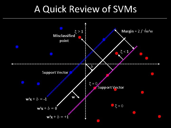
A Quick Review of SVMs Margin = 2 / wtw >1 Misclassified point < 1 b Support Vector = 0 wtx + b = -1 wtx + b = 0 wtx + b = +1 Support Vector w = 0

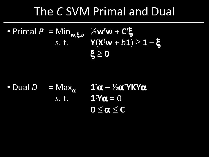
The C SVM Primal and Dual • Primal P = Minw, , b ½wtw + Ct s. t. Y(Xtw + b 1) 1 – 0 • Dual D = Max s. t. 1 t – ½ t. YKY 1 t. Y = 0 0 C

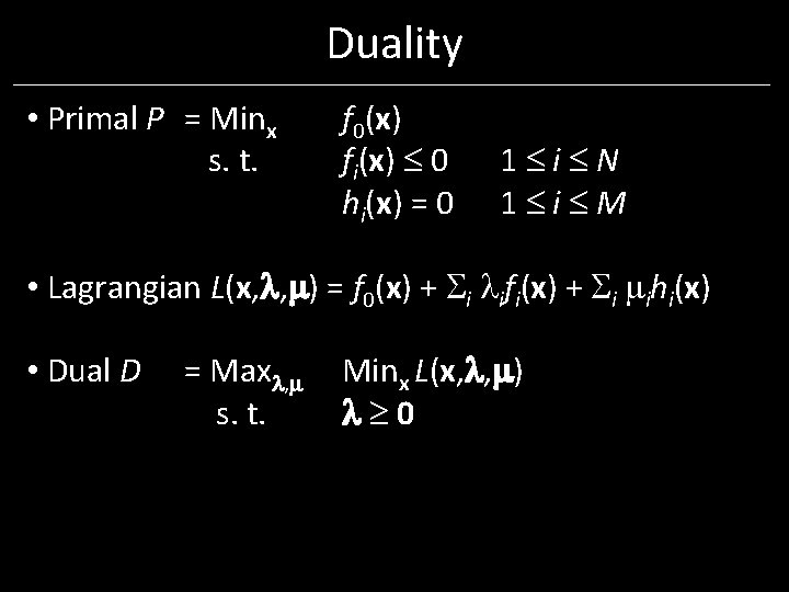
Duality • Primal P = Minx s. t. f 0(x) fi(x) 0 hi(x) = 0 1 i N 1 i M • Lagrangian L(x, , ) = f 0(x) + i ifi(x) + i ihi(x) • Dual D = Max , Minx L(x, , ) s. t. 0

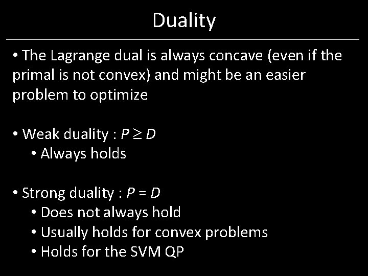
Duality • The Lagrange dual is always concave (even if the primal is not convex) and might be an easier problem to optimize • Weak duality : P D • Always holds • Strong duality : P = D • Does not always hold • Usually holds for convex problems • Holds for the SVM QP

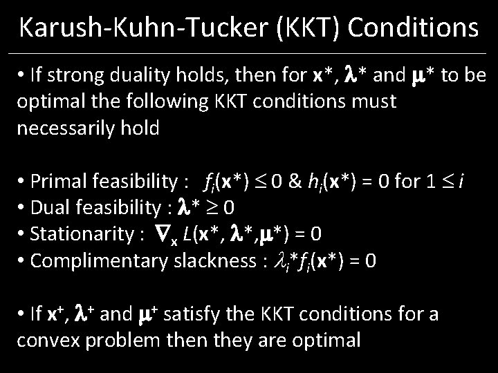
Karush-Kuhn-Tucker (KKT) Conditions • If strong duality holds, then for x*, * and * to be optimal the following KKT conditions must necessarily hold • Primal feasibility : fi(x*) 0 & hi(x*) = 0 for 1 i • Dual feasibility : * 0 • Stationarity : x L(x*, *, *) = 0 • Complimentary slackness : i*fi(x*) = 0 • If x+, + and + satisfy the KKT conditions for a convex problem then they are optimal

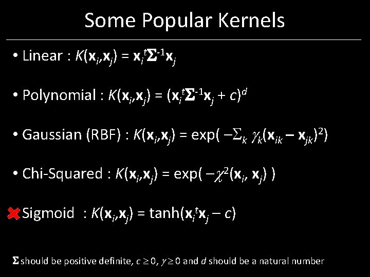
Some Popular Kernels • Linear : K(xi, xj) = xit -1 xj • Polynomial : K(xi, xj) = (xit -1 xj + c)d • Gaussian (RBF) : K(xi, xj) = exp( – k k(xik – xjk)2) • Chi-Squared : K(xi, xj) = exp( – 2(xi, xj) ) • Sigmoid : K(xi, xj) = tanh(xitxj – c) should be positive definite, c 0, 0 and d should be a natural number

Advantages of Learning the Kernel • Improve accuracy and generalization • Learn an RBF Kernel : K(xi, xj) = exp( – k (xik – xjk)2)

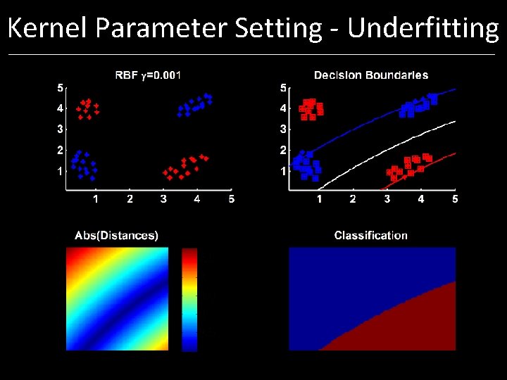
Kernel Parameter Setting - Underfitting

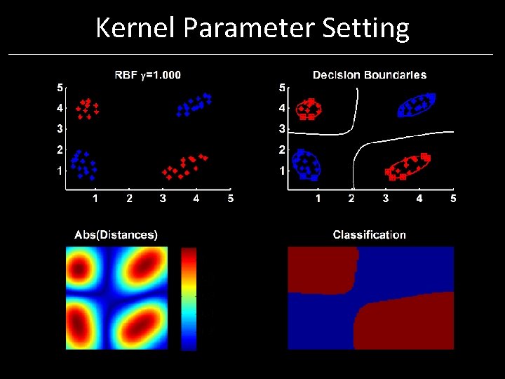
Kernel Parameter Setting

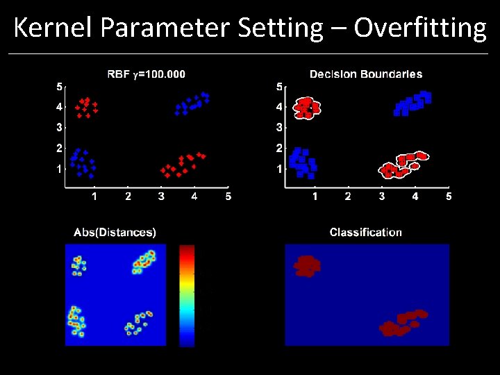
Kernel Parameter Setting – Overfitting

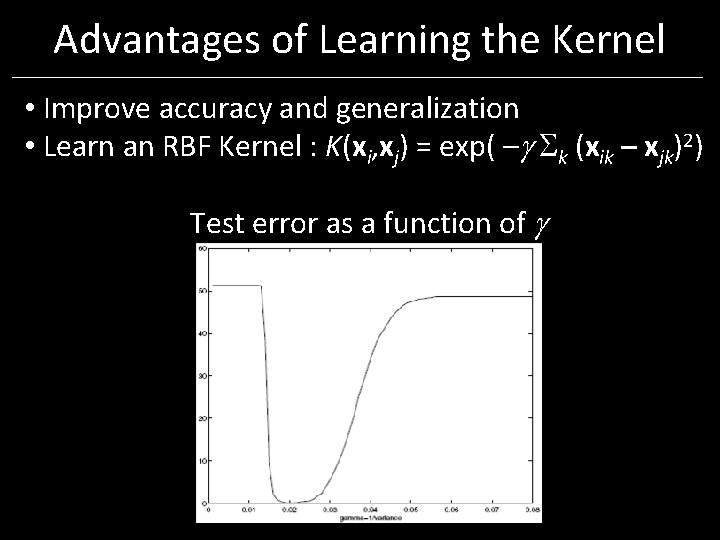
Advantages of Learning the Kernel • Improve accuracy and generalization • Learn an RBF Kernel : K(xi, xj) = exp( – k (xik – xjk)2) Test error as a function of

Advantages of Learning the Kernel • Perform non-linear feature selection • Learn an RBF Kernel : K(xi, xj) = exp(– k k(xik – xjk)2) • Perform non-linear dimensionality reduction • Learn K(P xi, P xj) where P is a low dimensional projection matrix parameterized by • These are optimized for the task at hand such as classification, regression, ranking, etc.

Advantages of Learning the Kernel • Multiple Kernel Learning • Learn a linear combination of given base kernels • K(xi, xj) = k dk Kk(xi, xj) • Can be used to combine heterogeneous sources of data • Can be used for descriptor (feature) selection

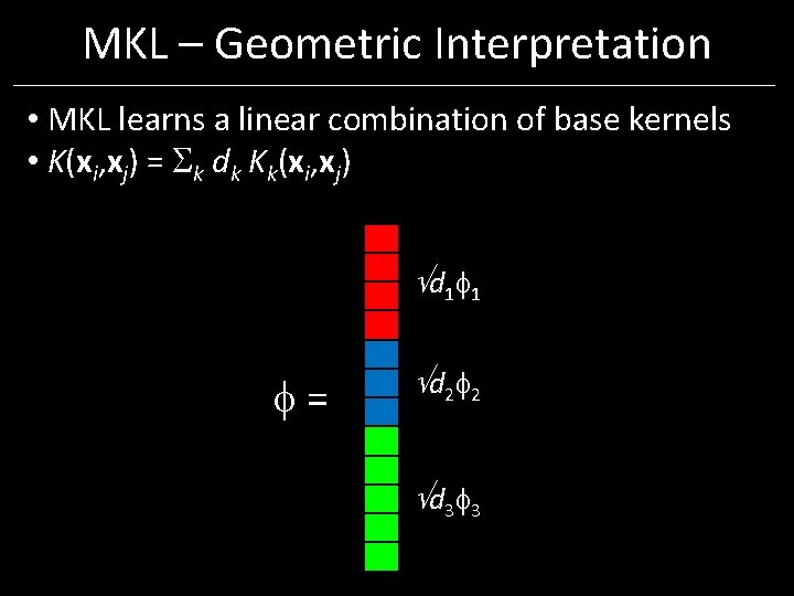
MKL – Geometric Interpretation • MKL learns a linear combination of base kernels • K(xi, xj) = k dk Kk(xi, xj) d 1 1 = d 2 2 d 3 3

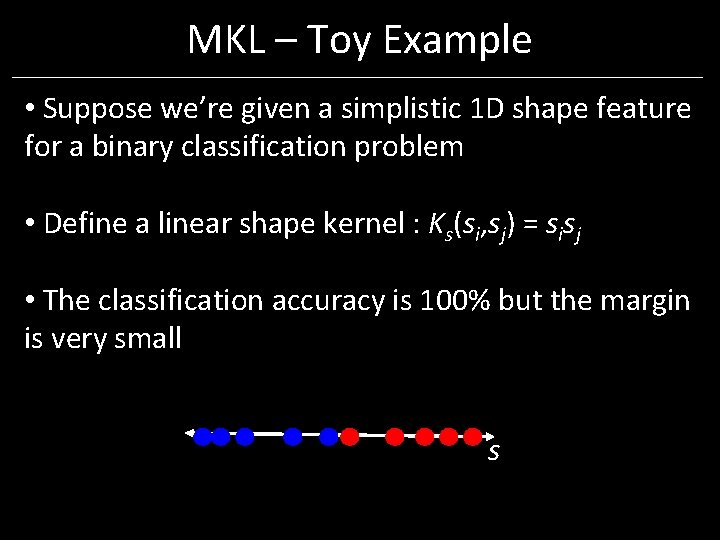
MKL – Toy Example • Suppose we’re given a simplistic 1 D shape feature for a binary classification problem • Define a linear shape kernel : Ks(si, sj) = sisj • The classification accuracy is 100% but the margin is very small s

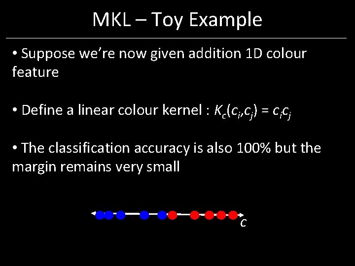
MKL – Toy Example • Suppose we’re now given addition 1 D colour feature • Define a linear colour kernel : Kc(ci, cj) = cicj • The classification accuracy is also 100% but the margin remains very small c

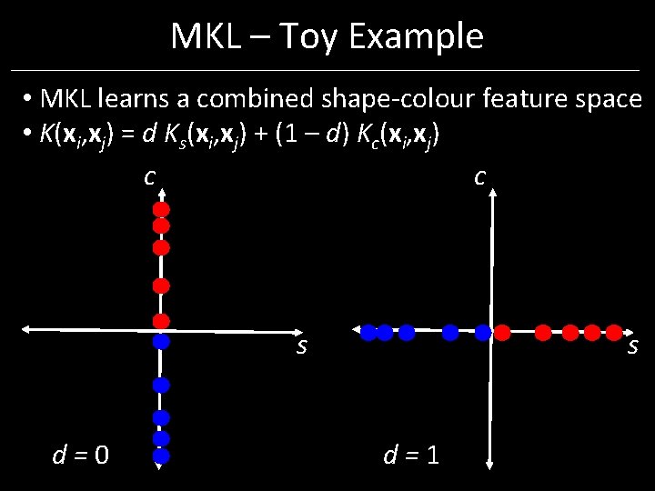
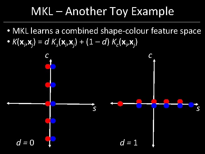
MKL – Toy Example • MKL learns a combined shape-colour feature space • K(xi, xj) = d Ks(xi, xj) + (1 – d) Kc(xi, xj) c c s d=0 s d=1

MKL – Toy Example

MKL – Another Toy Example • MKL learns a combined shape-colour feature space • K(xi, xj) = d Ks(xi, xj) + (1 – d) Kc(xi, xj) c c s d=0 s d=1

MKL – Another Toy Example

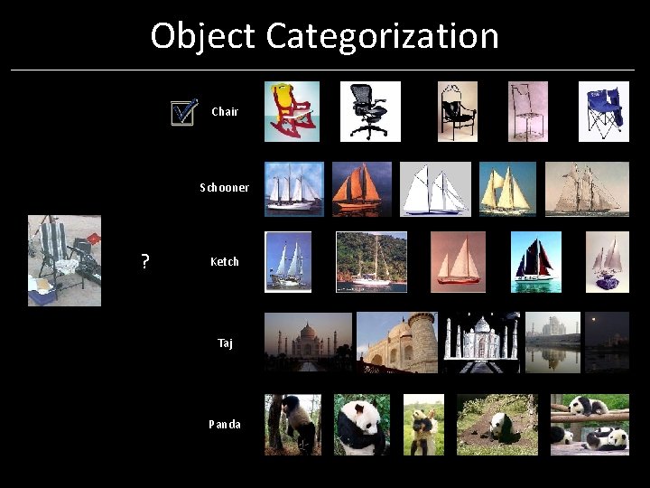
Object Categorization Chair Schooner ? Ketch Taj Panda

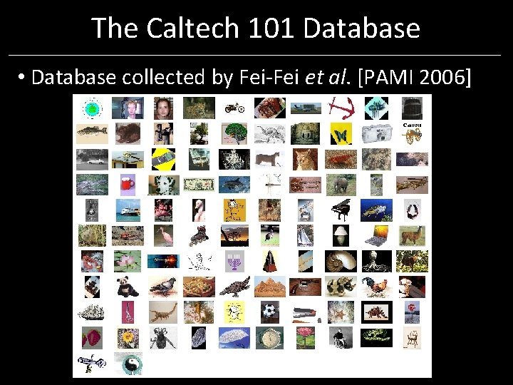
The Caltech 101 Database • Database collected by Fei-Fei et al. [PAMI 2006]

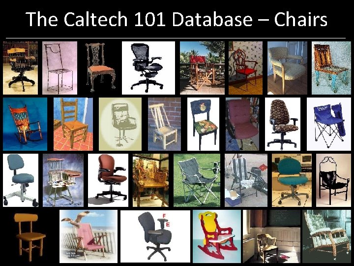
The Caltech 101 Database – Chairs

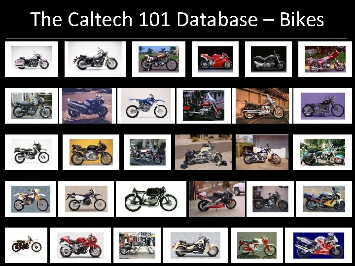
The Caltech 101 Database – Bikes

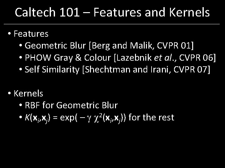
Caltech 101 – Features and Kernels • Features • Geometric Blur [Berg and Malik, CVPR 01] • PHOW Gray & Colour [Lazebnik et al. , CVPR 06] • Self Similarity [Shechtman and Irani, CVPR 07] • Kernels • RBF for Geometric Blur • K(xi, xj) = exp( – 2(xi, xj)) for the rest

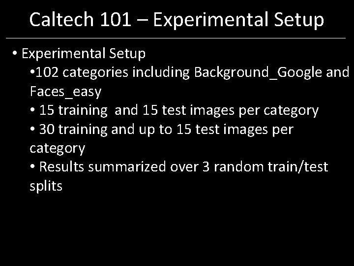
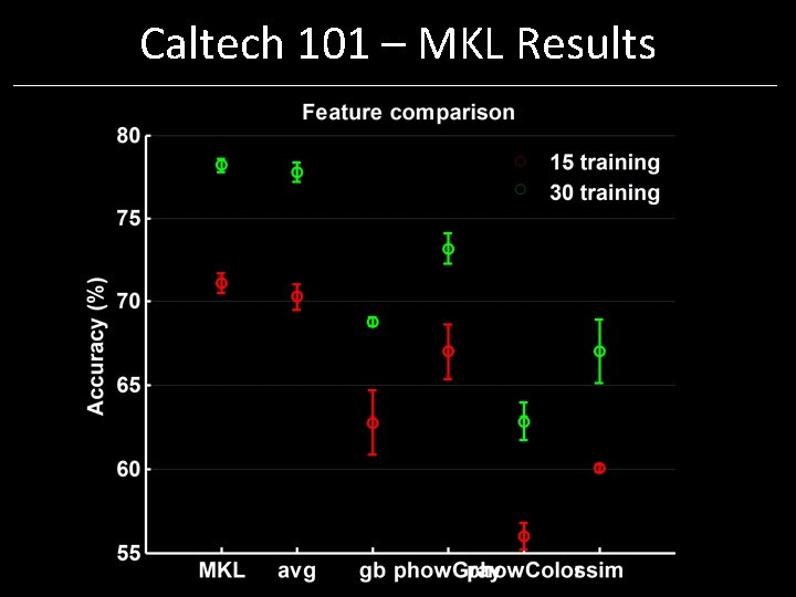
Caltech 101 – Experimental Setup • 102 categories including Background_Google and Faces_easy • 15 training and 15 test images per category • 30 training and up to 15 test images per category • Results summarized over 3 random train/test splits

Caltech 101 – MKL Results

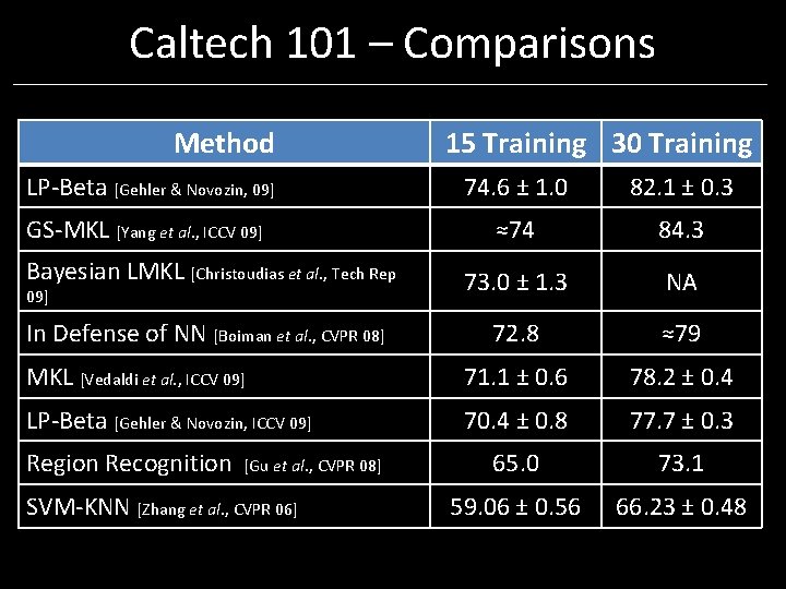
Caltech 101 – Comparisons Method 15 Training 30 Training LP-Beta [Gehler & Novozin, 09] 74. 6 ± 1. 0 82. 1 ± 0. 3 GS-MKL [Yang et al. , ICCV 09] ≈74 84. 3 Bayesian LMKL [Christoudias et al. , Tech Rep 73. 0 ± 1. 3 NA In Defense of NN [Boiman et al. , CVPR 08] 72. 8 ≈79 MKL [Vedaldi et al. , ICCV 09] 71. 1 ± 0. 6 78. 2 ± 0. 4 LP-Beta [Gehler & Novozin, ICCV 09] 70. 4 ± 0. 8 77. 7 ± 0. 3 65. 0 73. 1 59. 06 ± 0. 56 66. 23 ± 0. 48 09] Region Recognition [Gu et al. , CVPR 08] SVM-KNN [Zhang et al. , CVPR 06]

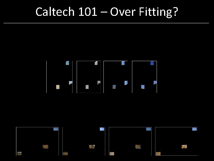
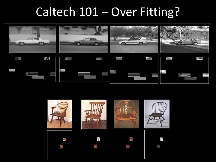
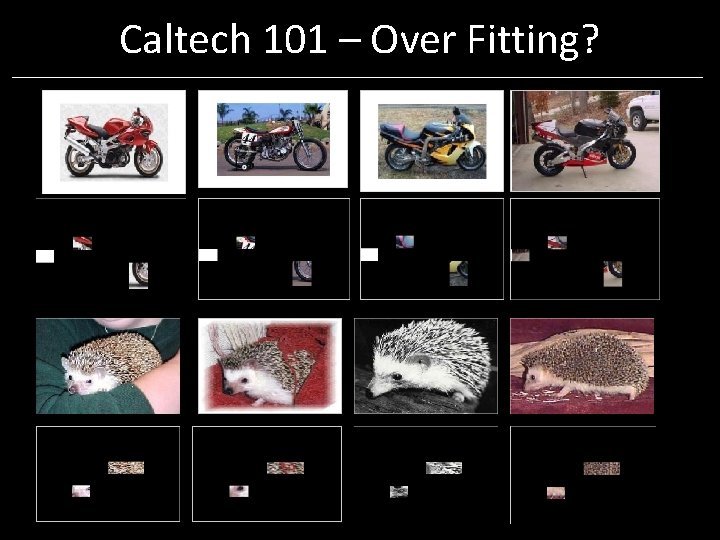
Caltech 101 – Over Fitting?

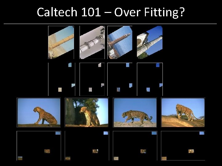
Caltech 101 – Over Fitting?

Caltech 101 – Over Fitting?

Caltech 101 – Over Fitting?

Caltech 101 – Over Fitting?

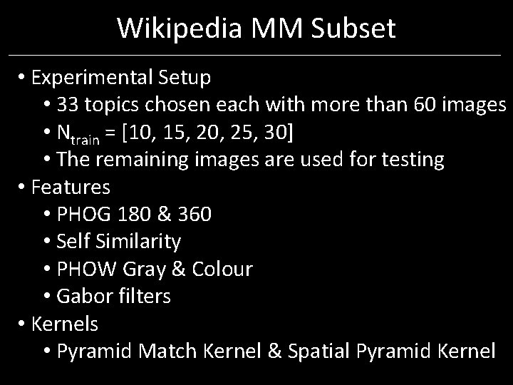
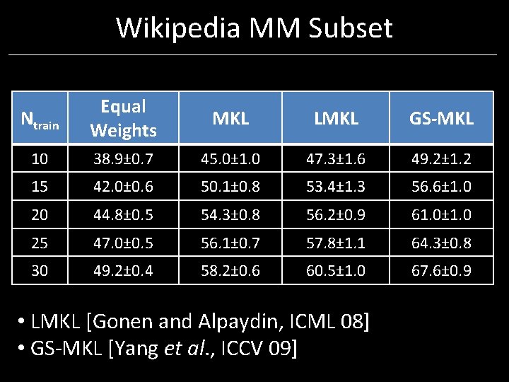
Wikipedia MM Subset • Experimental Setup • 33 topics chosen each with more than 60 images • Ntrain = [10, 15, 20, 25, 30] • The remaining images are used for testing • Features • PHOG 180 & 360 • Self Similarity • PHOW Gray & Colour • Gabor filters • Kernels • Pyramid Match Kernel & Spatial Pyramid Kernel

Wikipedia MM Subset Ntrain Equal Weights MKL LMKL GS-MKL 10 38. 9± 0. 7 45. 0± 1. 0 47. 3± 1. 6 49. 2± 1. 2 15 42. 0± 0. 6 50. 1± 0. 8 53. 4± 1. 3 56. 6± 1. 0 20 44. 8± 0. 5 54. 3± 0. 8 56. 2± 0. 9 61. 0± 1. 0 25 47. 0± 0. 5 56. 1± 0. 7 57. 8± 1. 1 64. 3± 0. 8 30 49. 2± 0. 4 58. 2± 0. 6 60. 5± 1. 0 67. 6± 0. 9 • LMKL [Gonen and Alpaydin, ICML 08] • GS-MKL [Yang et al. , ICCV 09]

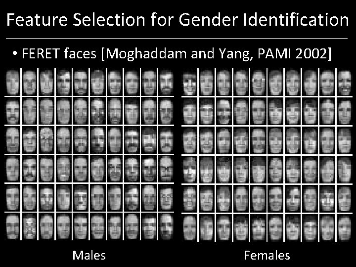
Feature Selection for Gender Identification • FERET faces [Moghaddam and Yang, PAMI 2002] Males Females

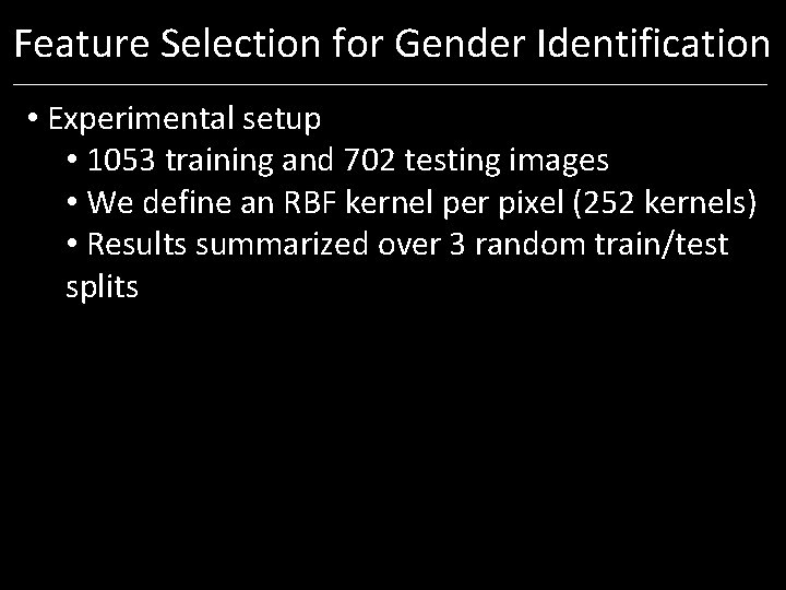
Feature Selection for Gender Identification • Experimental setup • 1053 training and 702 testing images • We define an RBF kernel per pixel (252 kernels) • Results summarized over 3 random train/test splits

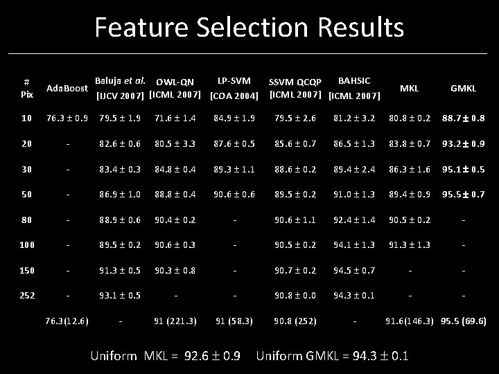
Feature Selection Results Baluja et al. OWL-QN LP-SVM BAHSIC SSVM QCQP [IJCV 2007] [ICML 2007] [COA 2004] [ICML 2007] # Pix Ada. Boost 10 76. 3 0. 9 79. 5 1. 9 71. 6 1. 4 84. 9 1. 9 79. 5 2. 6 20 - 82. 6 0. 6 80. 5 3. 3 87. 6 0. 5 30 - 83. 4 0. 3 84. 8 0. 4 50 - 86. 9 1. 0 80 - 100 MKL GMKL 81. 2 3. 2 80. 8 0. 2 88. 7 0. 8 85. 6 0. 7 86. 5 1. 3 83. 8 0. 7 93. 2 0. 9 89. 3 1. 1 88. 6 0. 2 89. 4 2. 4 86. 3 1. 6 95. 1 0. 5 88. 8 0. 4 90. 6 89. 5 0. 2 91. 0 1. 3 89. 4 0. 9 95. 5 0. 7 88. 9 0. 6 90. 4 0. 2 - 90. 6 1. 1 92. 4 1. 4 90. 5 0. 2 - - 89. 5 0. 2 90. 6 0. 3 - 90. 5 0. 2 94. 1 1. 3 91. 3 - 150 - 91. 3 0. 5 90. 3 0. 8 - 90. 7 0. 2 94. 5 0. 7 - - 252 - 93. 1 0. 5 - - 90. 8 0. 0 94. 3 0. 1 - - 76. 3(12. 6) - 91 (221. 3) 91 (58. 3) 90. 8 (252) - 91. 6(146. 3) 95. 5 (69. 6) Uniform MKL = 92. 6 0. 9 Uniform GMKL = 94. 3 0. 1

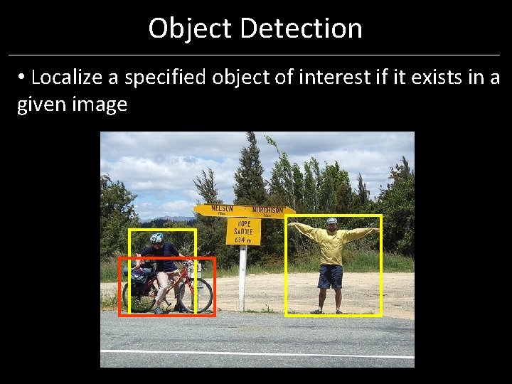
Object Detection • Localize a specified object of interest if it exists in a given image

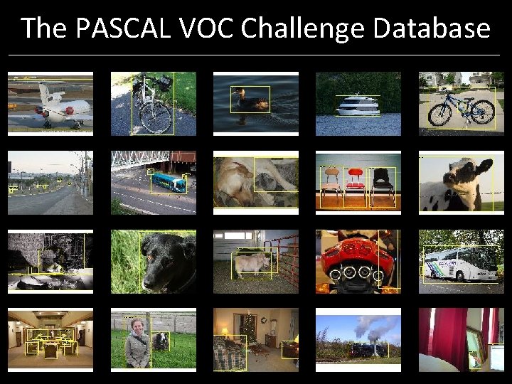
The PASCAL VOC Challenge Database

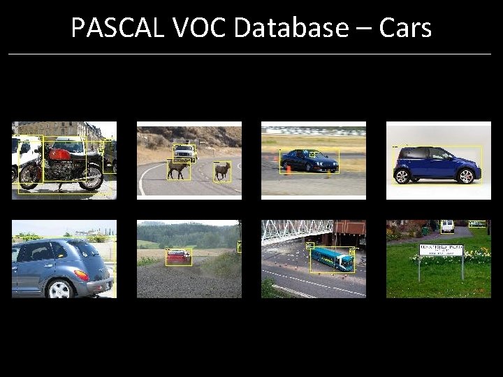
PASCAL VOC Database – Cars

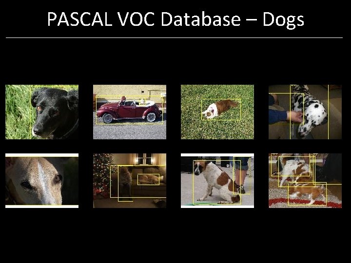
PASCAL VOC Database – Dogs

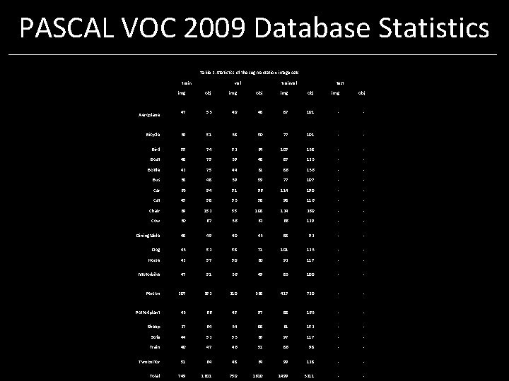
PASCAL VOC 2009 Database Statistics Table 2: Statistics of the segmentation image sets. Aeroplane Bicycle train Table 1: Statistics of the main image sets. Object statistics list val trainval only the `non-difficult' objects used in the evaluation. img obj train img val obj trainval img testobj img obj 47 39 Bird 55 Boat 48 Bottle 42 Bus 38 Car 63 Cat 45 Chair 69 Cow 30 Diningtable 48 Dog 43 Horse 42 Motorbike 47 Person 207 Aerop lane Bicycl e Bird Boat Bottle Bus Car Cat Chair Cow Dining table Dog Horse Motor bike Perso n Potte dplant Sheep Sofa Train Tvmo nitor Total 53 201 267 167 51 262 74170 220 75 132 75372 266 48 338 94 86 232 40 206 407 87 533 - - - - 243 155 200 126 358 277 330 86 505 325 420 258 730 543 668 172 468 77 760 537 107 787 87 365 1317 86 622 77 1429 114 336 58140 153 53 131 58 153 271 98 306 - 116 - - - 152316 67161 391 55 333 237 36 167 108 392 245 62 649 124 783 328 482 66 - 260 - 129 - - - - 171 235 167 234 338 469 49 40 43 88 1333 2819 1446 2996 2779 5815 52 166 57 67 51155 164 311 58 50 166 163 64 172 36 153 190 160 71 316 60 175 49 191 101 627 92 131 338 308 347 83 324 381 332 180 259 173 257 353 516 352 210 368 417 3473 8505 3581 8713 7054 17218 101 - 138 123 - 136 107 - 190 - - obj 348 381 270 52 394 39 179 664 44 308 39 716 164 51 - 101 img 236 50 379 267 64 393 48 186 653 61 314 59 713 96 172 38 181 48 266 test - 92 - 123 117 - - 100 - 720 - - Pottedplant 43 66 45 97 88 163 - - Sheep 27 64 34 88 61 152 - - Sofa 44 52 53 65 97 117 - - Train 40 47 46 51 86 98 - - Tvmonitor 51 64 48 64 99 128 - - Total 749 1601 750 1610 1499 3211 - -

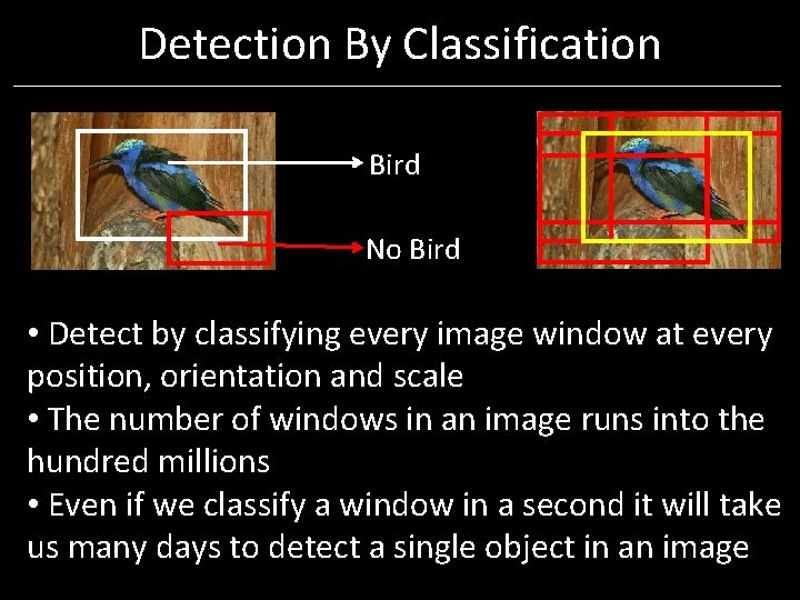
Detection By Classification Bird No Bird • Detect by classifying every image window at every position, orientation and scale • The number of windows in an image runs into the hundred millions • Even if we classify a window in a second it will take us many days to detect a single object in an image

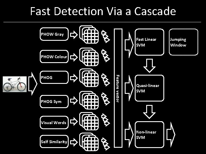
Fast Detection Via a Cascade PHOW Gray Fast Linear SVM PHOW Colour PHOG Sym Feature vector PHOG Quasi-linear SVM Visual Words Self Similarity Non-linear SVM Jumping Window

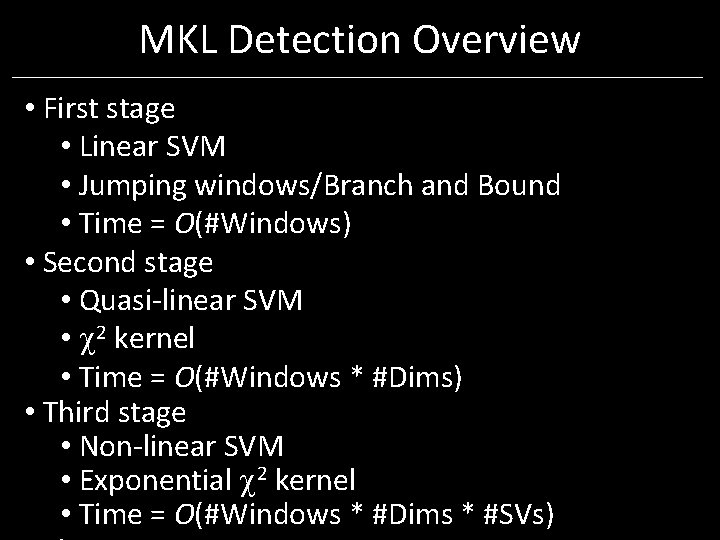
MKL Detection Overview • First stage • Linear SVM • Jumping windows/Branch and Bound • Time = O(#Windows) • Second stage • Quasi-linear SVM • 2 kernel • Time = O(#Windows * #Dims) • Third stage • Non-linear SVM • Exponential 2 kernel • Time = O(#Windows * #Dims * #SVs)

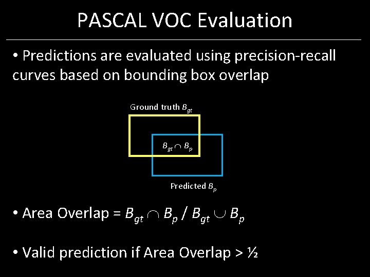
PASCAL VOC Evaluation • Predictions are evaluated using precision-recall curves based on bounding box overlap Ground truth Bgt Bp Predicted Bp • Area Overlap = Bgt Bp / Bgt Bp • Valid prediction if Area Overlap > ½

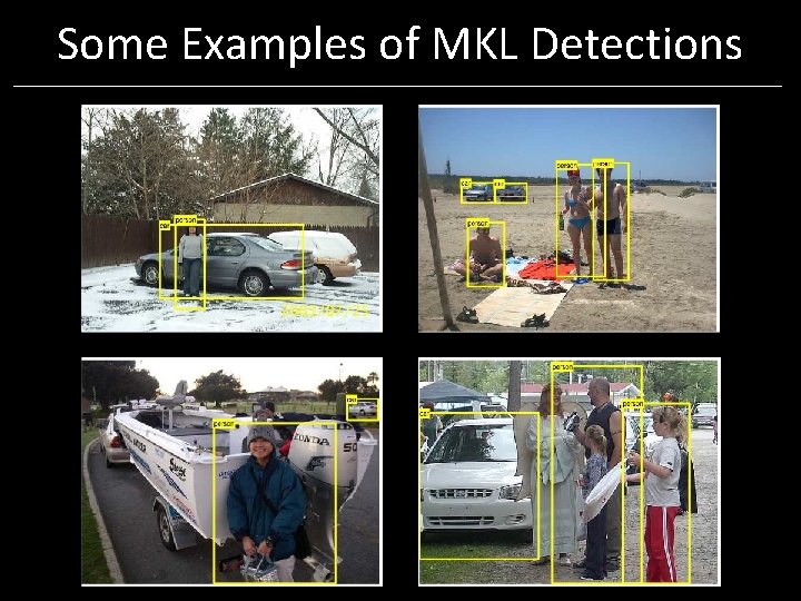
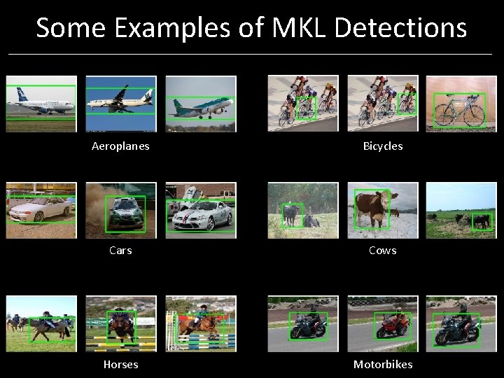
Some Examples of MKL Detections

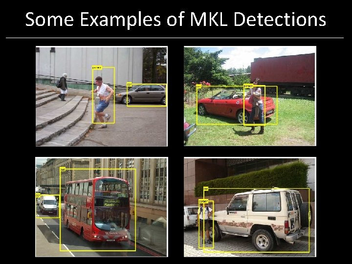
Some Examples of MKL Detections

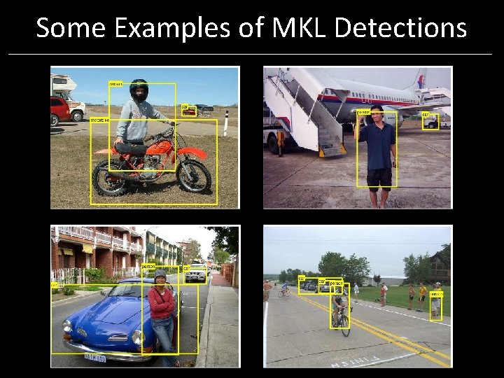
Some Examples of MKL Detections

Some Examples of MKL Detections Aeroplanes Bicycles Cars Cows Horses Motorbikes

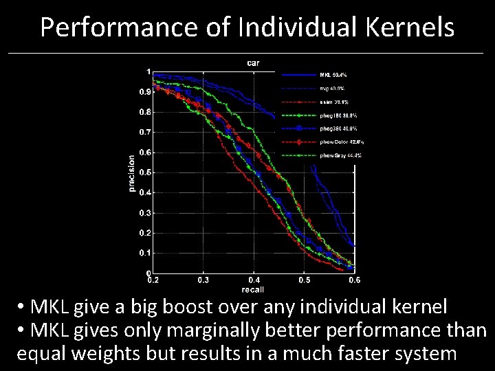
Performance of Individual Kernels • MKL give a big boost over any individual kernel • MKL gives only marginally better performance than equal weights but results in a much faster system

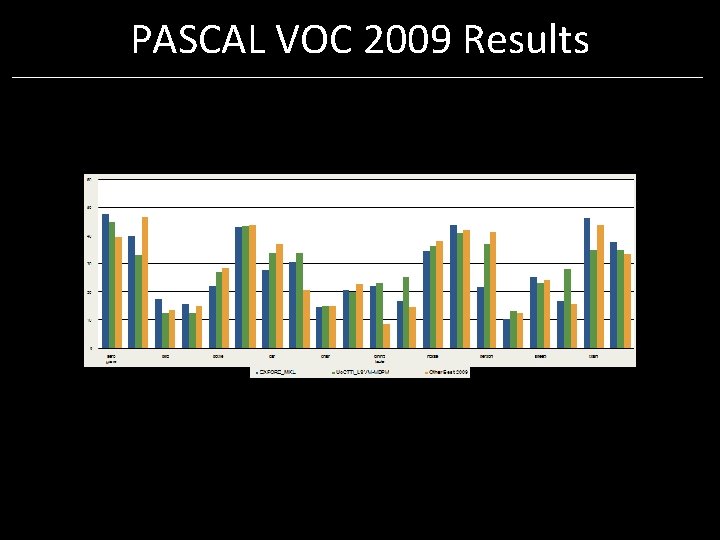
PASCAL VOC 2009 Results

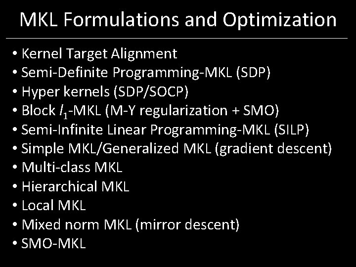
MKL Formulations and Optimization • Kernel Target Alignment • Semi-Definite Programming-MKL (SDP) • Hyper kernels (SDP/SOCP) • Block l 1 -MKL (M-Y regularization + SMO) • Semi-Infinite Linear Programming-MKL (SILP) • Simple MKL/Generalized MKL (gradient descent) • Multi-class MKL • Hierarchical MKL • Local MKL • Mixed norm MKL (mirror descent) • SMO-MKL

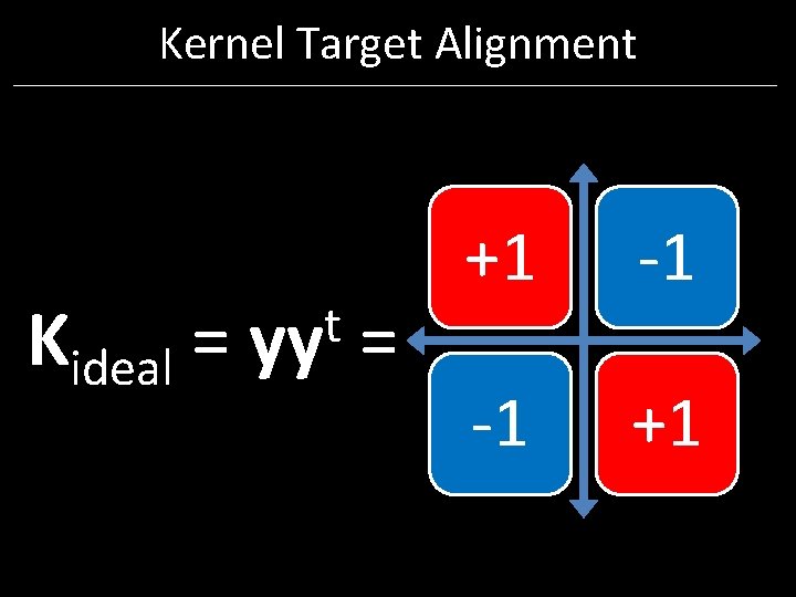
Kernel Target Alignment Kideal t = yy = +1 -1 -1 +1

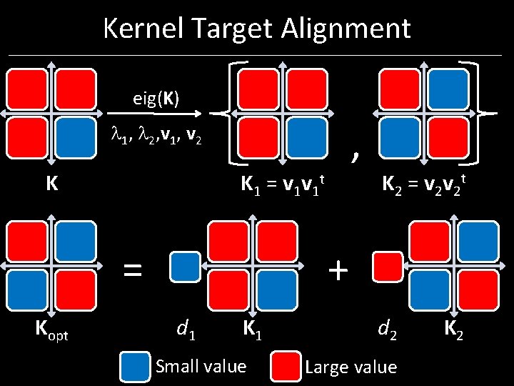
Kernel Target Alignment eig(K) 1, 2, v 1, v 2 K K 1 = v 1 v 1 t Kopt , = d 1 K 1 Small value + K 2 = v 2 v 2 t d 2 Large value K 2

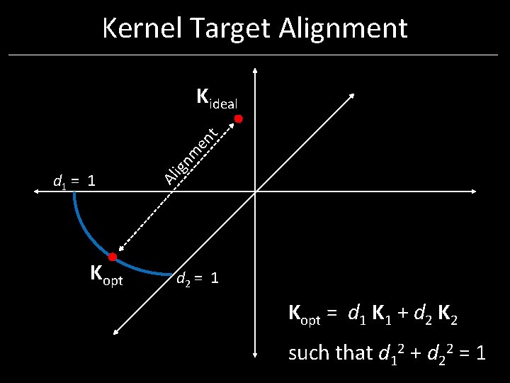
Kernel Target Alignment d 1 = 1 Kopt Al ign m en t Kideal d 2 = 1 Kopt = d 1 K 1 + d 2 K 2 such that d 12 + d 22 = 1

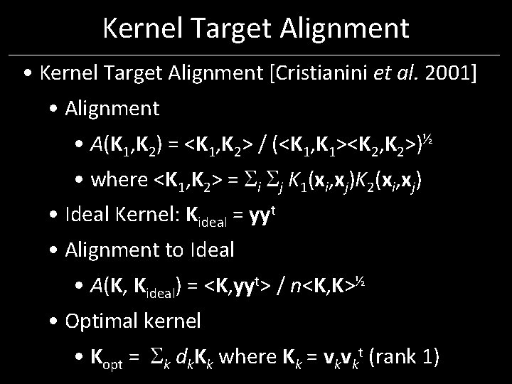
Kernel Target Alignment • Kernel Target Alignment [Cristianini et al. 2001] • Alignment • A(K 1, K 2) = <K 1, K 2> / (<K 1, K 1><K 2, K 2>)½ • where <K 1, K 2> = i j K 1(xi, xj)K 2(xi, xj) • Ideal Kernel: Kideal = yyt • Alignment to Ideal • A(K, Kideal) = <K, yyt> / n<K, K>½ • Optimal kernel • Kopt = k dk. Kk where Kk = vkvkt (rank 1)

Kernel Target Alignment • Optimal Alignment: • A(Kopt) = dk<vk, y>2 / n( dk 2)½ • Assume dk 2 = 1 • Lagrangian • L( , d) = dk<vk, y>2 – ( dk 2 – 1) • Optimal weights: dk <vk, y>2

Kernel Target Alignment • One of the first papers to propose kernel learning. • Established taking linear combinations of base kernels • Efficient algorithm • Formulation based on l 2 regularization. • Some generalisation bounds have been given but the task is not directly related to classification • Does not easily generalize to other loss functions

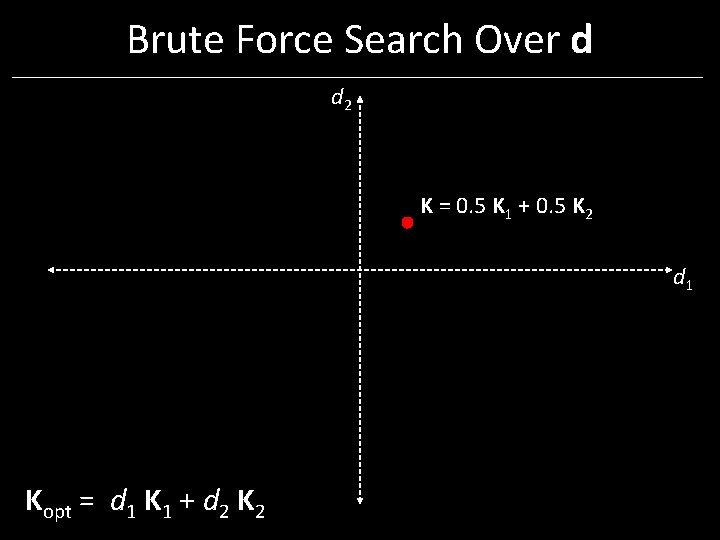
Brute Force Search Over d d 2 K = 0. 5 K 1 + 0. 5 K 2 d 1 Kopt = d 1 K 1 + d 2 K 2

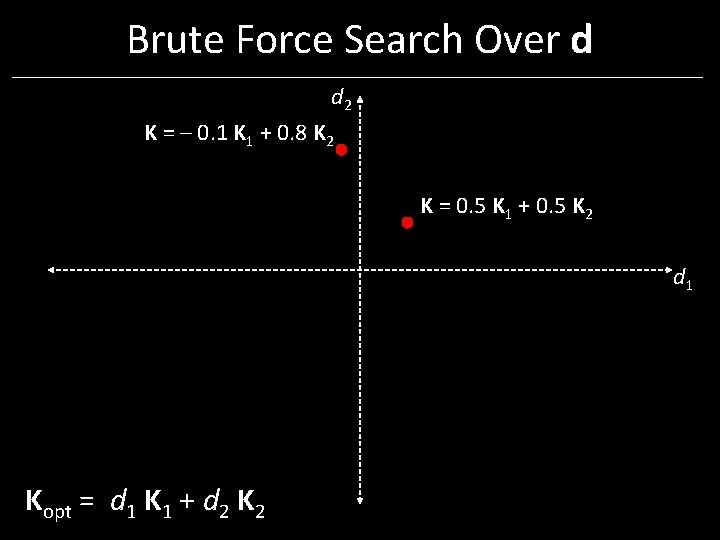
Brute Force Search Over d d 2 K = – 0. 1 K 1 + 0. 8 K 2 K = 0. 5 K 1 + 0. 5 K 2 d 1 Kopt = d 1 K 1 + d 2 K 2

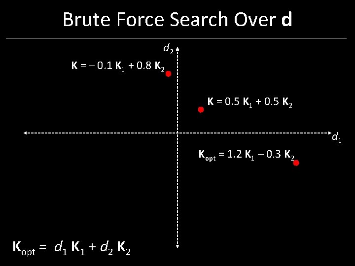
Brute Force Search Over d d 2 K = – 0. 1 K 1 + 0. 8 K 2 K = 0. 5 K 1 + 0. 5 K 2 d 1 Kopt = 1. 2 K 1 – 0. 3 K 2 Kopt = d 1 K 1 + d 2 K 2

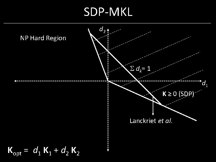
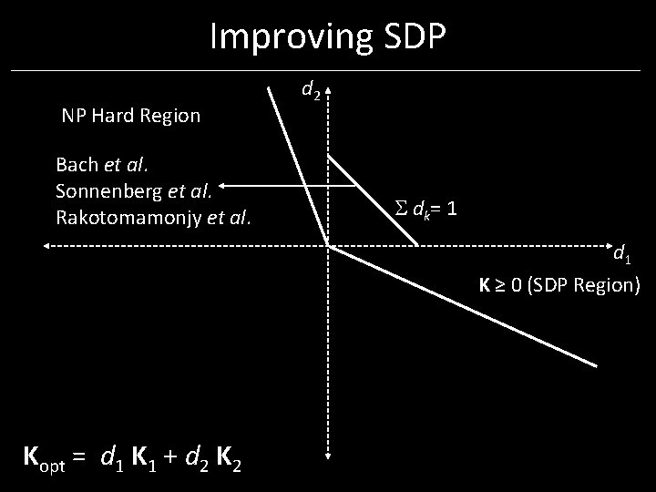
SDP-MKL NP Hard Region d 2 dk= 1 d 1 K ≥ 0 (SDP) Lanckriet et al. Kopt = d 1 K 1 + d 2 K 2

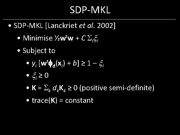
SDP-MKL • SDP-MKL [Lanckriet et al. 2002] • Minimise ½wtw + C i i • Subject to • yi [wt d(xi) + b] ≥ 1 – i • i ≥ 0 • K = k dk. Kk ≥ 0 (positive semi-definite) • trace(K) = constant

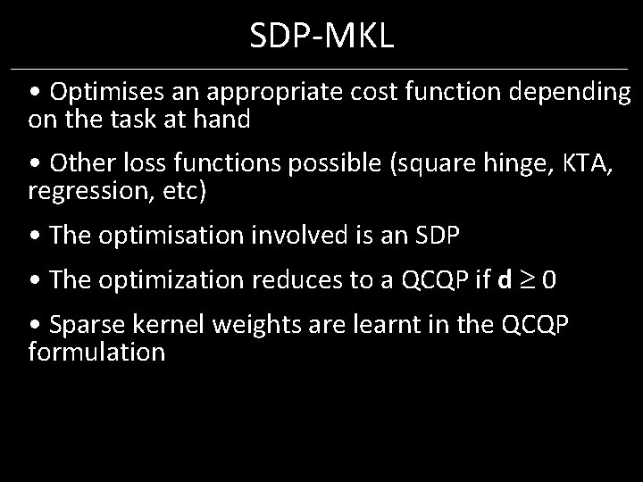
SDP-MKL • Optimises an appropriate cost function depending on the task at hand • Other loss functions possible (square hinge, KTA, regression, etc) • The optimisation involved is an SDP • The optimization reduces to a QCQP if d 0 • Sparse kernel weights are learnt in the QCQP formulation

Improving SDP NP Hard Region Bach et al. Sonnenberg et al. Rakotomamonjy et al. d 2 dk= 1 d 1 K ≥ 0 (SDP Region) Kopt = d 1 K 1 + d 2 K 2

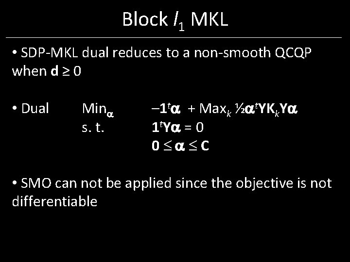
Block l 1 MKL • SDP-MKL dual reduces to a non-smooth QCQP when d ≥ 0 • Dual Min s. t. – 1 t + Maxk ½ t. YKk. Y 1 t. Y = 0 0 C • SMO can not be applied since the objective is not differentiable

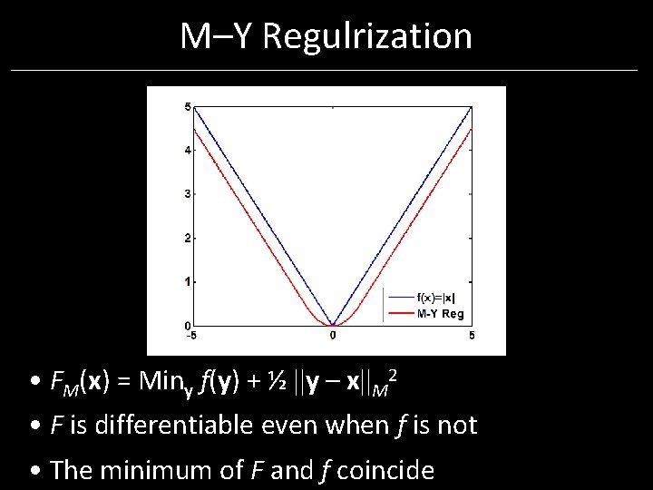
M–Y Regulrization • FM(x) = Miny f(y) + ½ ||y – x||M 2 • F is differentiable even when f is not • The minimum of F and f coincide

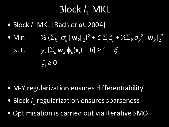
Block l 1 MKL • Block l 1 MKL [Bach et al. 2004] • Min ½ ( k k ||wk||2)2 + C i i + ½ k ak 2 ||wk||22 s. t. yi [ k wkt k(xi) + b] ≥ 1 – i i ≥ 0 • M-Y regularization ensures differentiability • Block l 1 regularization ensures sparseness • Optimisation is carried out via iterative SMO

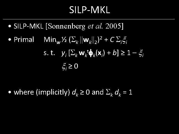
SILP-MKL • SILP-MKL [Sonnenberg et al. 2005] • Primal Minw ½ ( k ||wk||2)2 + C i i s. t. yi [ k wkt k(xi) + b] ≥ 1 – i i ≥ 0 • where (implicitly) dk ≥ 0 and k dk = 1

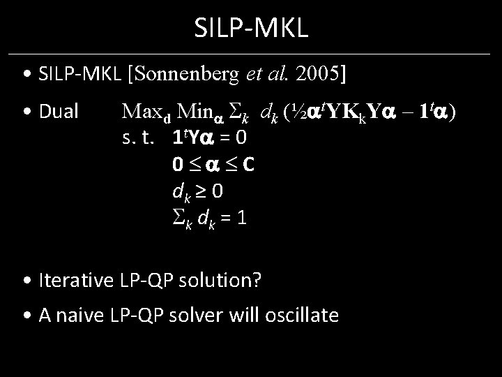
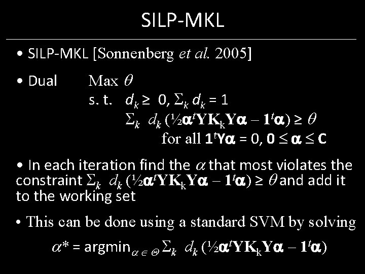
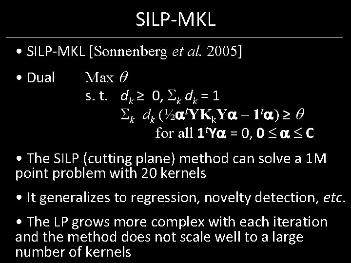
SILP-MKL • SILP-MKL [Sonnenberg et al. 2005] • Dual Maxd Min k dk (½ t. YKk. Y – 1 t ) s. t. 1 t. Y = 0 0 C dk ≥ 0 k dk = 1 • Iterative LP-QP solution? • A naive LP-QP solver will oscillate

SILP-MKL • SILP-MKL [Sonnenberg et al. 2005] • Dual Max s. t. dk ≥ 0, k dk = 1 k dk (½ t. YKk. Y – 1 t ) ≥ for all 1 t. Y = 0, 0 C • In each iteration find the that most violates the constraint k dk (½ t. YKk. Y – 1 t ) ≥ and add it to the working set • This can be done using a standard SVM by solving * = argmin k dk (½ t. YKk. Y – 1 t )

SILP-MKL • SILP-MKL [Sonnenberg et al. 2005] • Dual Max s. t. dk ≥ 0, k dk = 1 k dk (½ t. YKk. Y – 1 t ) ≥ for all 1 t. Y = 0, 0 C • The SILP (cutting plane) method can solve a 1 M point problem with 20 kernels • It generalizes to regression, novelty detection, etc. • The LP grows more complex with each iteration and the method does not scale well to a large number of kernels

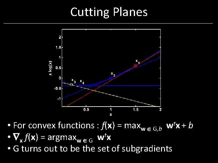
Cutting Planes • For convex functions : f(x) = maxw G, b wtx + b • x f(x) = argmaxw G wtx • G turns out to be the set of subgradients

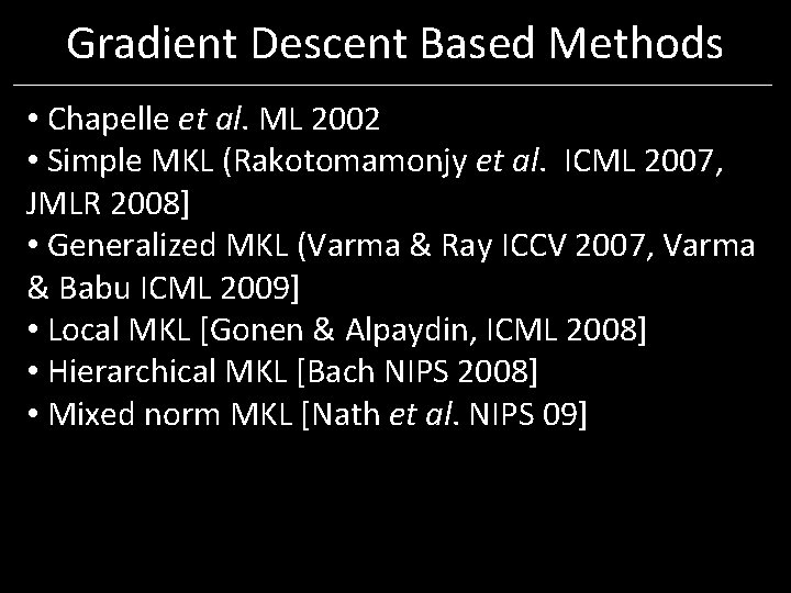
Gradient Descent Based Methods • Chapelle et al. ML 2002 • Simple MKL (Rakotomamonjy et al. ICML 2007, JMLR 2008] • Generalized MKL (Varma & Ray ICCV 2007, Varma & Babu ICML 2009] • Local MKL [Gonen & Alpaydin, ICML 2008] • Hierarchical MKL [Bach NIPS 2008] • Mixed norm MKL [Nath et al. NIPS 09]

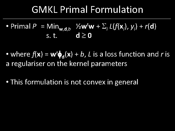
GMKL Primal Formulation • Primal P = Minw, d, b ½wtw + i L(f(xi), yi) + r(d) s. t. d 0 • where f(x) = wt d(x) + b, L is a loss function and r is a regulariser on the kernel parameters • This formulation is not convex in general

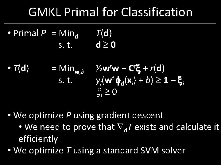
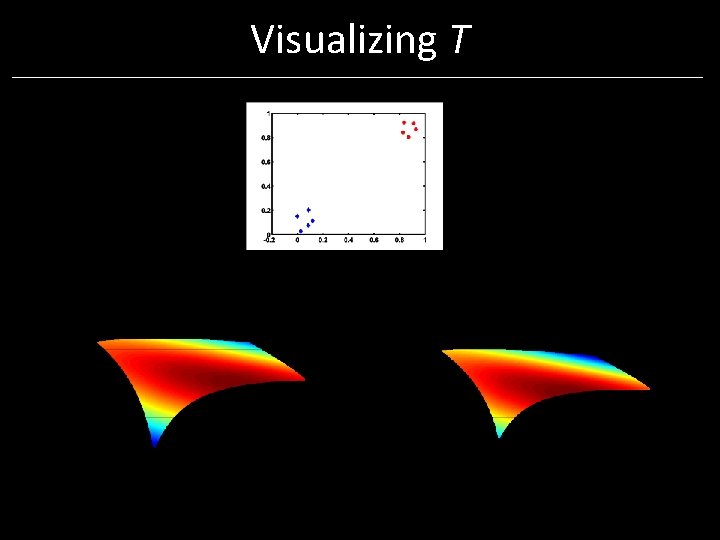
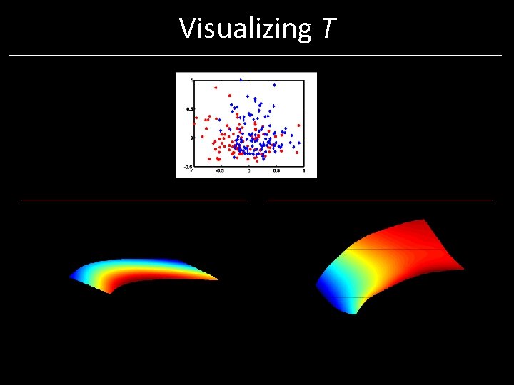
GMKL Primal for Classification • Primal P = Mind s. t. • T(d) d 0 = Minw, b ½wtw + Ct + r(d) s. t. yi(wt d(xi) + b) 1 – i i 0 • We optimize P using gradient descent • We need to prove that d. T exists and calculate it efficiently • We optimize T using a standard SVM solver

Visualizing T

Visualizing T

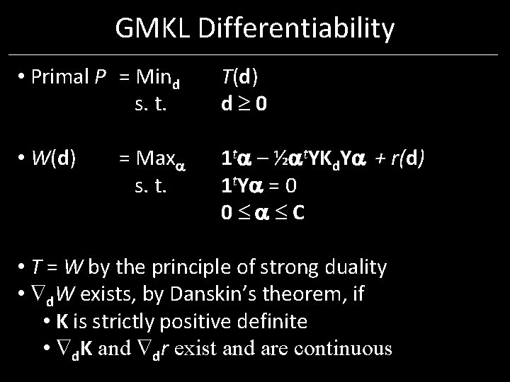
GMKL Differentiability • Primal P = Mind s. t. T(d) d 0 • W(d) 1 t – ½ t. YKd. Y + r(d) 1 t. Y = 0 0 C = Max s. t. • T = W by the principle of strong duality • d. W exists, by Danskin’s theorem, if • K is strictly positive definite • d. K and dr exist and are continuous

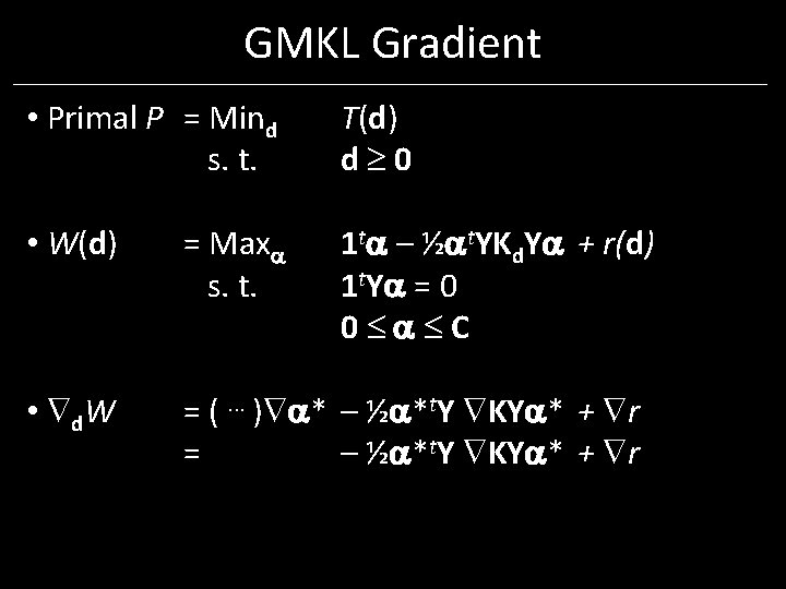
GMKL Gradient • Primal P = Mind s. t. T(d) d 0 • W(d) = Max s. t. 1 t – ½ t. YKd. Y + r(d) 1 t. Y = 0 0 C • d. W = (. . . ) * – ½ *t. Y KY * + r = – ½ *t. Y KY * + r

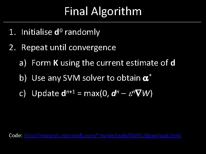
Final Algorithm 1. Initialise d 0 randomly 2. Repeat until convergence a) Form K using the current estimate of d b) Use any SVM solver to obtain * c) Update dn+1 = max(0, dn – n W) Code: http: //research. microsoft. com/~manik/code/GMKL/download. html

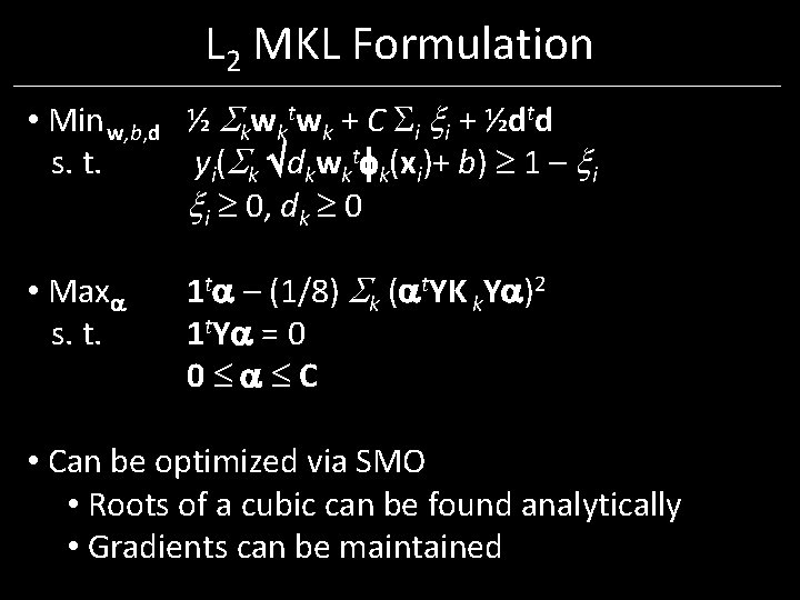
L 2 MKL Formulation • Min w, b, d ½ kwktwk + C i i + ½dtd s. t. yi( k dkwkt k(xi)+ b) 1 – i i 0, dk 0 • Max s. t. 1 t – (1/8) k ( t. YK k. Y )2 1 t. Y = 0 0 C • Can be optimized via SMO • Roots of a cubic can be found analytically • Gradients can be maintained