Image Restoration using Auto encoding Priors Siavash Arjomand

Image Restoration using Auto -encoding Priors Siavash Arjomand, Matthias Zwicker

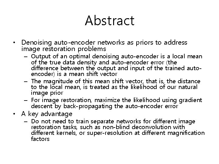
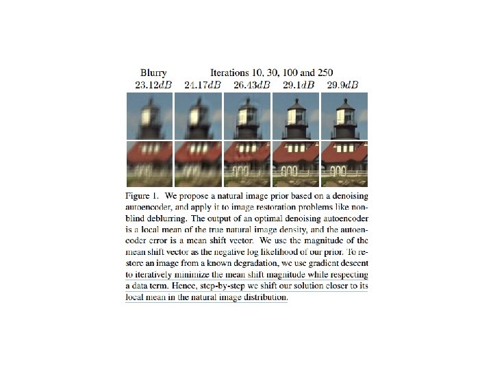
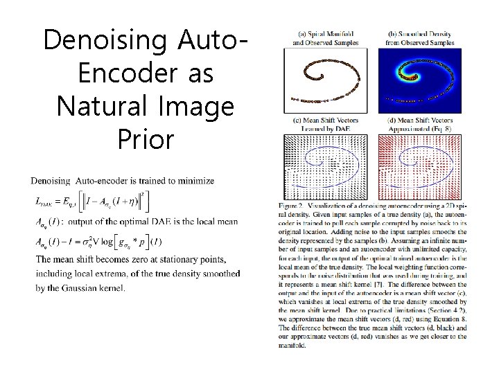
Abstract • Denoising auto-encoder networks as priors to address image restoration problems – Output of an optimal denoising auto-encoder is a local mean of the true data density and auto-encoder error (the difference between the output and input of the trained autoencoder) is a mean shift vector – The magnitude of this mean shift vector, that is, the distance to the local mean, is treated as the likelihood of our natural image prior – For image restoration, maximize the likelihood using gradient descent by back-propagating the auto-encoder error • A key advantage – Do not need to train separate networks for different image restoration tasks, such as non-blind deconvolution with different kernels, or super-resolution at different magnification factors

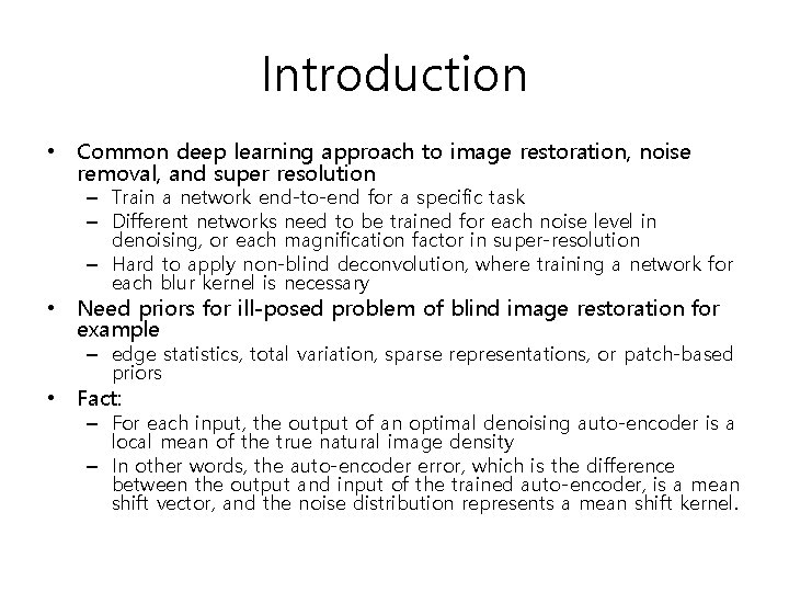
Introduction • Common deep learning approach to image restoration, noise removal, and super resolution – Train a network end-to-end for a specific task – Different networks need to be trained for each noise level in denoising, or each magnification factor in super-resolution – Hard to apply non-blind deconvolution, where training a network for each blur kernel is necessary • Need priors for ill-posed problem of blind image restoration for example – edge statistics, total variation, sparse representations, or patch-based priors • Fact: – For each input, the output of an optimal denoising auto-encoder is a local mean of the true natural image density – In other words, the auto-encoder error, which is the difference between the output and input of the trained auto-encoder, is a mean shift vector, and the noise distribution represents a mean shift kernel.

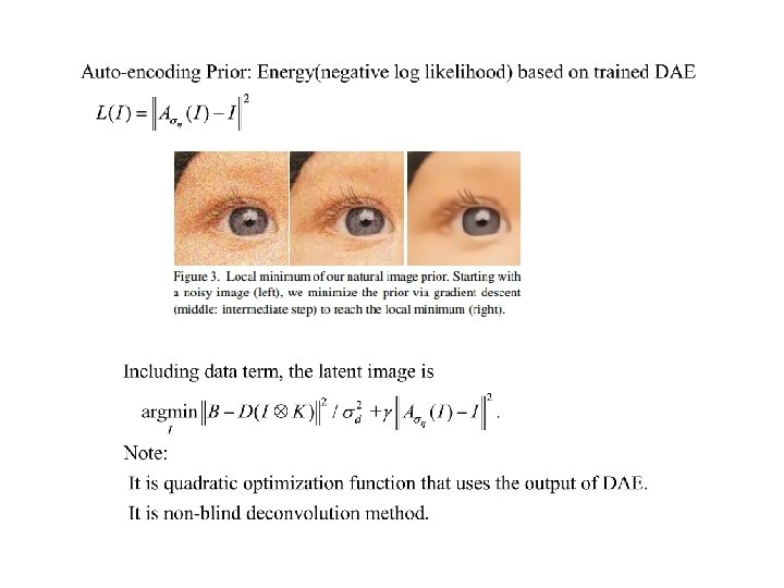
• Propose denoising auto-encoder (DAE) networks as natural image priors – Given the trained auto-encoder, the prior is based on the magnitude of the mean shift vector – For each image, the mean shift is proportional to the gradient of the true data distribution smoothed by the mean shift kernel, and its magnitude is the distance to the local mean in the distribution of natural images – With an optimal DAE, the energy of the prior vanishes exactly at the stationary points of the true data distribution smoothed by the mean shift kernel – This makes the prior attractive for maximum a posteriori (MAP) estimation • Objective function of MAP – Data term + Prior of mean shift error from DAE – Minimize the objective function • Minimize the mean shift error by back-propagation and the gradient of the data term

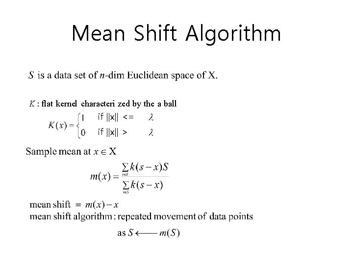
Mean Shift Algorithm K : flat kernel characteri zed by the a ball if ||x|| <= if ||x|| >

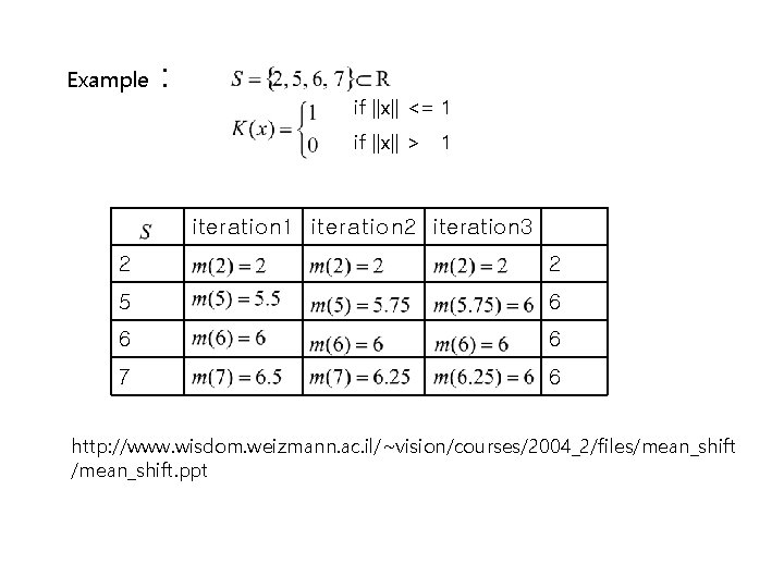
Example : if ||x|| <= 1 if ||x|| > 1 iteration 2 iteration 3 2 2 5 6 6 6 7 6 http: //www. wisdom. weizmann. ac. il/~vision/courses/2004_2/files/mean_shift. ppt

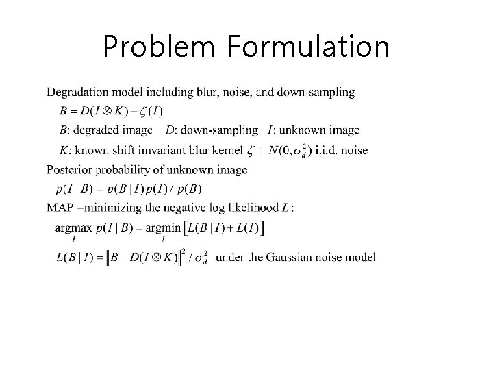
Problem Formulation

Denoising Auto. Encoder as Natural Image Prior

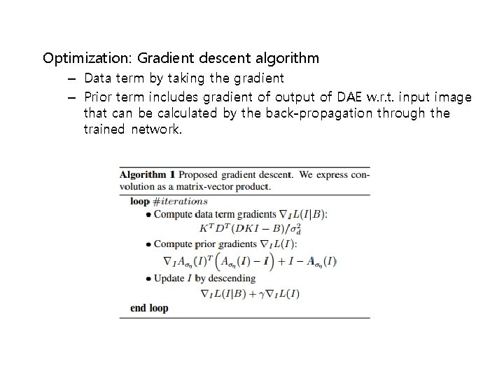
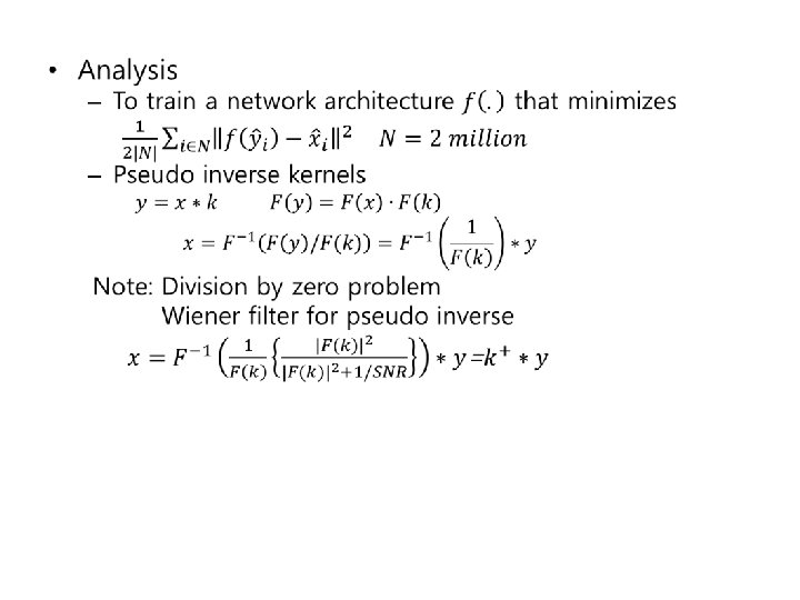
Optimization: Gradient descent algorithm – Data term by taking the gradient – Prior term includes gradient of output of DAE w. r. t. input image that can be calculated by the back-propagation through the trained network.

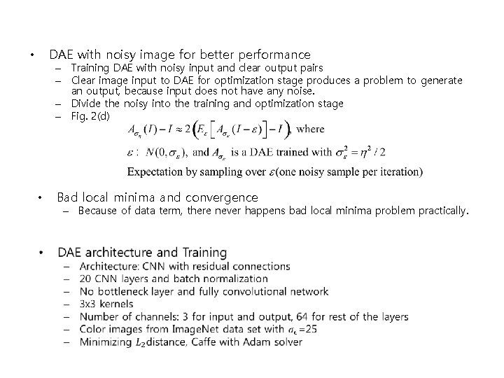
DAE with noisy image for better performance • – Training DAE with noisy input and clear output pairs – Clear image input to DAE for optimization stage produces a problem to generate an output, because input does not have any noise. – Divide the noisy into the training and optimization stage – Fig. 2(d) • Bad local minima and convergence – Because of data term, there never happens bad local minima problem practically.

Experimental Results

Convolutional Neural Networks for Direct Text Deblurring Michal Hradiš, Jan Kotera, Pavel Zemcík, and Filip Šroubek

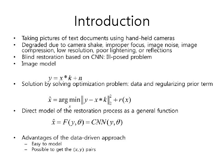
Introduction •

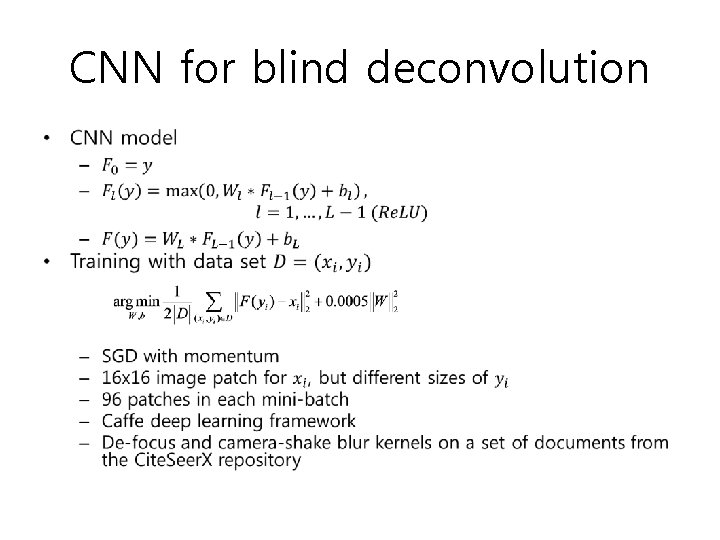
CNN for blind deconvolution •

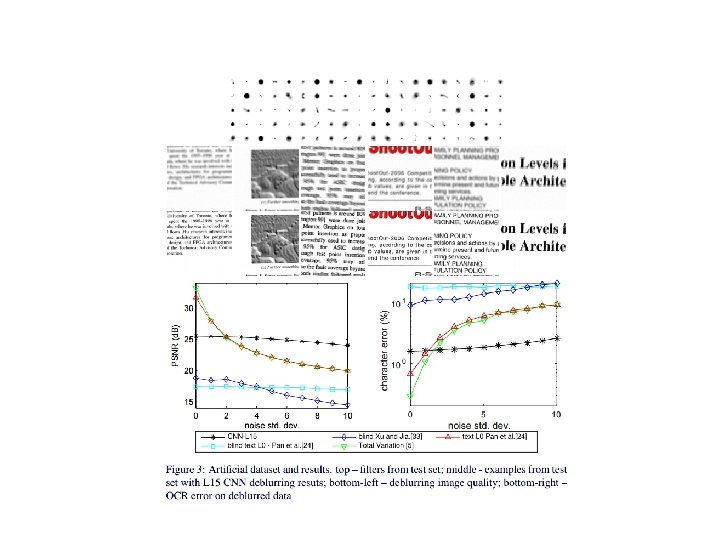
• Motion blur Maximum size of motion blur: sampled from [5, 21] Radius of de-focus blur: uniformly sampled from [5, 21] Each image patch was blurred with a unique kernel Histogram kernel size(see below fig. ) Gaussian noise with std. uniformly sampled [0, 7/255] was added and then quantized into 8 bits – Several CNN architectures were considered. – 3 M patches for training and 35 K for validation – – –

Learning a Convolutional Neural Network for Nonuniform Motion Blur Removal Jian Sun , Wenfei Cao , Zongben Xu , and Jean Ponce

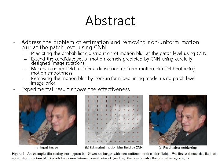
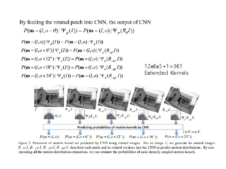
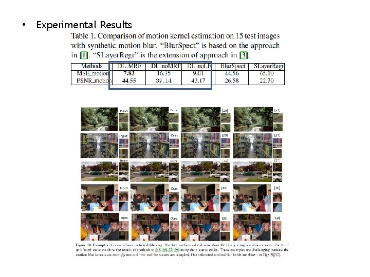
Abstract • Address the problem of estimation and removing non-uniform motion blur at the patch level using CNN – Predicting the probabilistic distribution of motion blur at the patch level using CNN – Extend the candidate set of motion kernels predicted by CNN using carefully designed image rotations – Markov random field to infer a dense non-uniform motion blur field enforcing motion smoothness – Removing the motion blur by non-uniform deblurring model using patch level image prior • Experimental result shows the effectiveness

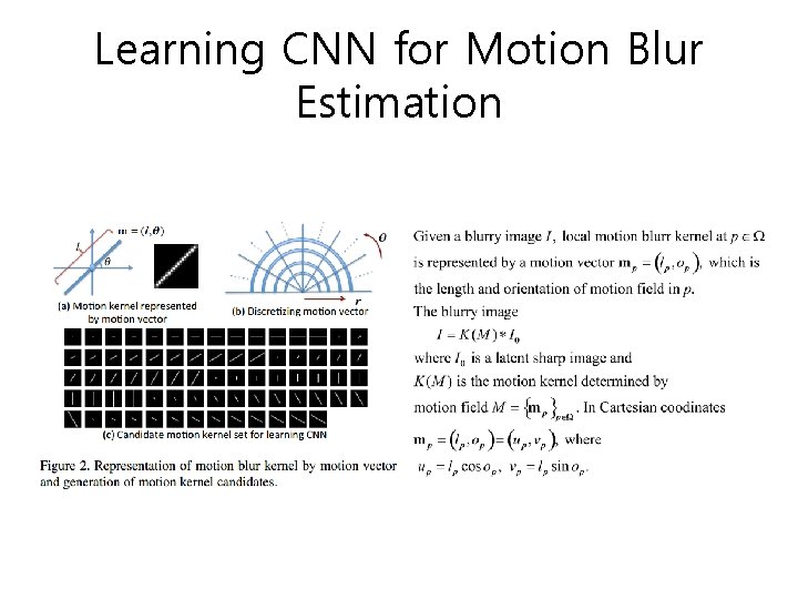
Learning CNN for Motion Blur Estimation

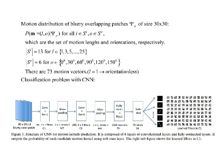
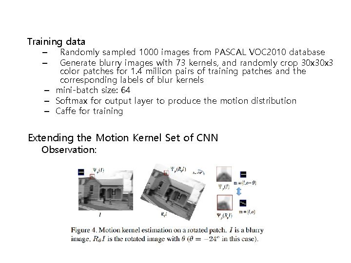
Training data Randomly sampled 1000 images from PASCAL VOC 2010 database Generate blurry images with 73 kernels, and randomly crop 30 x 3 color patches for 1. 4 million pairs of training patches and the corresponding labels of blur kernels – mini-batch size: 64 – Softmax for output layer to produce the motion distribution – Caffe for training – – Extending the Motion Kernel Set of CNN Observation:

12 x 6 x 5+1=361 Extended Kernels

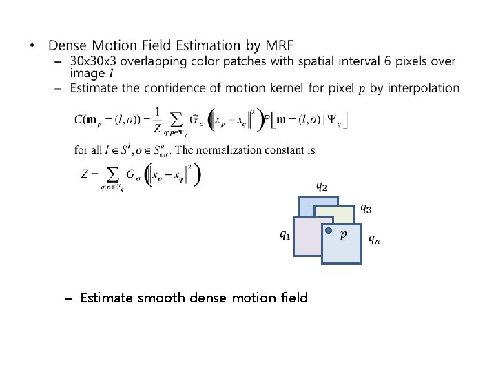
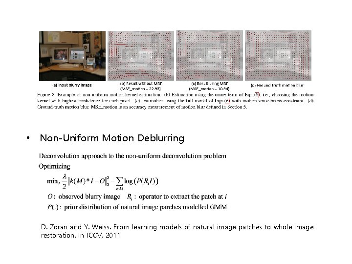
• – Estimate smooth dense motion field

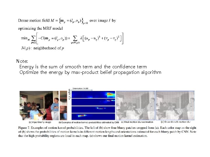
Note: Energy is the sum of smooth term and the confidence term Optimize the energy by max-product belief propagation algorithm

• Non-Uniform Motion Deblurring D. Zoran and Y. Weiss. From learning models of natural image patches to whole image restoration. In ICCV, 2011

• Experimental Results

Deep Convolutional Neural Network for Image Deconvolution Li Xu, Jimmy SJ. Ren Ce Liu, and Jiaya Jia

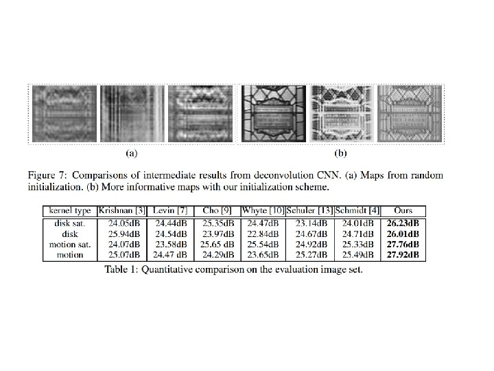
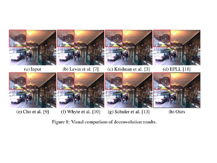
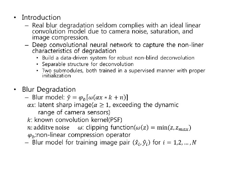
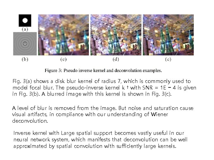
Fig. 3(a) shows a disk blur kernel of radius 7, which is commonly used to model focal blur. The pseudo-inverse kernel k † with SNR = 1 E − 4 is given in Fig. 3(b). A blurred image with this kernel is shown in Fig. 3(c). A level of blur is removed from the image. But noise and saturation cause visual artifacts, in compliance with our understanding of Wiener deconvolution. Inverse kernel with Large spatial support becomes vastly useful in our neural network system, which manifests that deconvolution can be well approximated by spatial convolution with sufficiently large kernels.

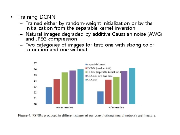
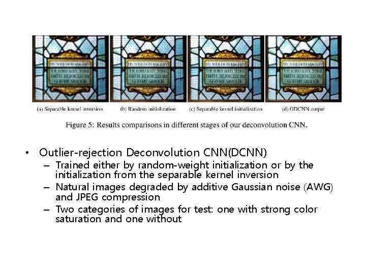
• Training DCNN – Trained either by random-weight initialization or by the initialization from the separable kernel inversion – Natural images degraded by additive Gaussian noise (AWG) and JPEG compression – Two categories of images for test: one with strong color saturation and one without

• Outlier-rejection Deconvolution CNN(DCNN) – Trained either by random-weight initialization or by the initialization from the separable kernel inversion – Natural images degraded by additive Gaussian noise (AWG) and JPEG compression – Two categories of images for test: one with strong color saturation and one without

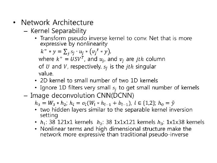
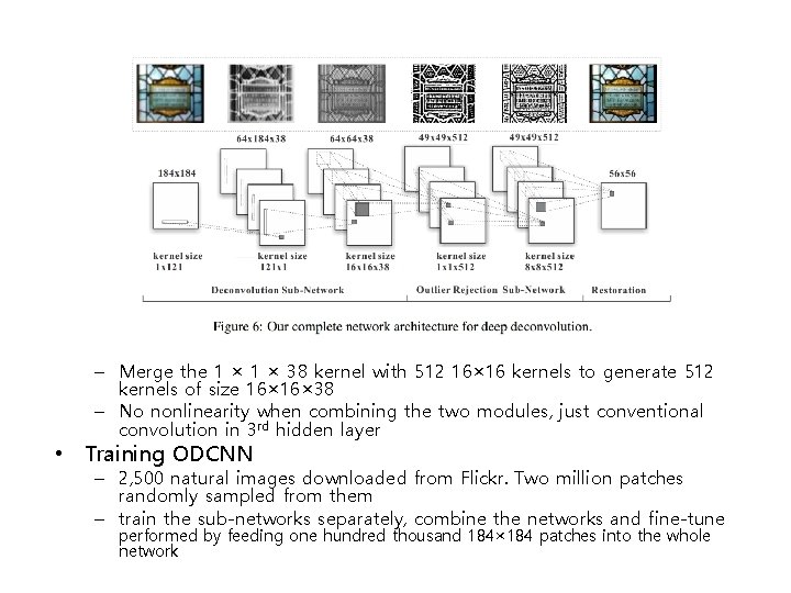
– Merge the 1 × 38 kernel with 512 16× 16 kernels to generate 512 kernels of size 16× 38 – No nonlinearity when combining the two modules, just conventional convolution in 3 rd hidden layer • Training ODCNN – 2, 500 natural images downloaded from Flickr. Two million patches randomly sampled from them – train the sub-networks separately, combine the networks and fine-tune performed by feeding one hundred thousand 184× 184 patches into the whole network