Lecture 10 Chapter 5 Image Restoration Image restoration

Lecture 10 Chapter 5: Image Restoration

Image restoration • Image restoration is the process of recovering the original scene from the observed scene which is degraded. • Different form enhancement- aim of enhancement techniques make images visually appealing, whereas restoration essentially inverts the degradation- more objective.

Image restoration • Has intersections with signal processing, estimation theory, inverse problems, linear algebra. • As with most of the topics in Image Processing, restoration was developed to be used in astronomy, and is also used for restoring old films and pictures

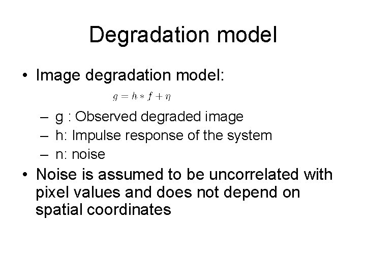
Degradation model • Image degradation model: – g : Observed degraded image – h: Impulse response of the system – n: noise • Noise is assumed to be uncorrelated with pixel values and does not depend on spatial coordinates

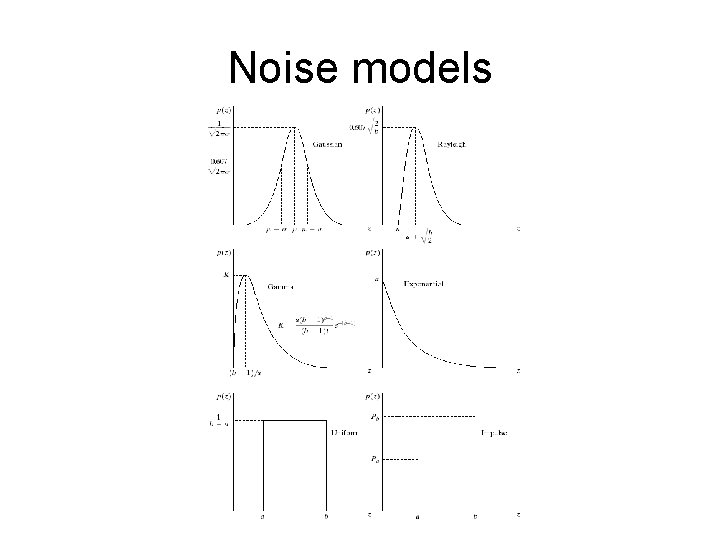
Noise models • Noise is characterized by its probability density function. Some of which are: • Gaussian, Rayleigh, Uniform, Exponential, etc. • By far Gaussian is the most popular model, because: – It is present widely in practice – Mathematical ease

Noise models

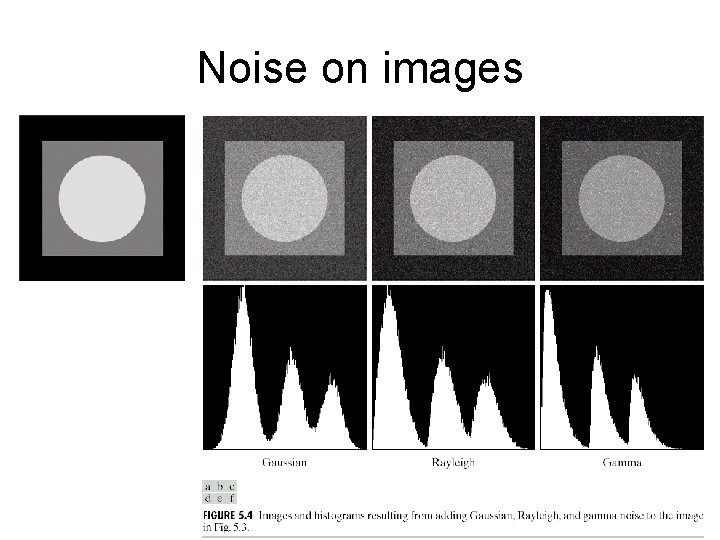
Noise on images

Identifying noise model • If the imaging system is available we can capture images of a uniform gray value object, example a black board uniformly illuminated. • If images from the system are given, look for part of images which are uniform.

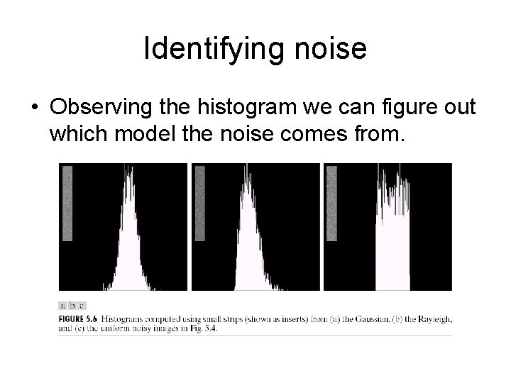
Identifying noise • Observing the histogram we can figure out which model the noise comes from.

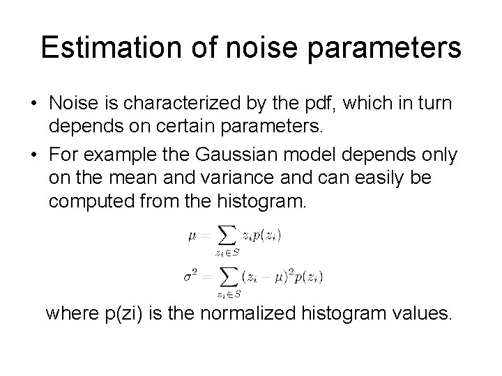
Estimation of noise parameters • Noise is characterized by the pdf, which in turn depends on certain parameters. • For example the Gaussian model depends only on the mean and variance and can easily be computed from the histogram. where p(zi) is the normalized histogram values.

Restoration in presence of noise • Degradation model: g = f + n • Restoration = Enhancement – Mean filtering, Median filtering, Notch filters. • Some new ones: – Geometric mean filter, Harmonic mean filters, Midpoint filter, etc.

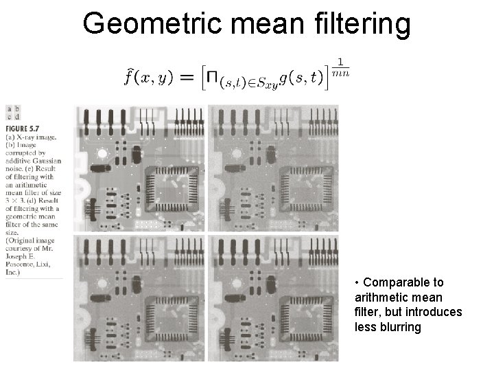
Geometric mean filtering • Comparable to arithmetic mean filter, but introduces less blurring

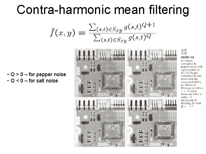
Contra-harmonic mean filtering • Q > 0 – for pepper noise • Q < 0 – for salt noise

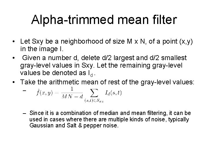
Alpha-trimmed mean filter • Let Sxy be a neighborhood of size M x N, of a point (x, y) in the image I. • Given a number d, delete d/2 largest and d/2 smallest gray-level values in Sxy. Let the remaining gray-level values be denoted as Id. • Take the arithmetic mean of rest of the gray-level values: – – Since it is a combination of median and mean filtering, it can be used in cases where there are multiple kinds of noise, typically Gaussian and Salt & pepper noise.

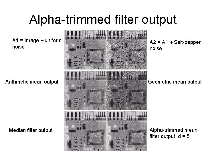
Alpha-trimmed filter output A 1 = Image + uniform noise A 2 = A 1 + Salt-pepper noise Arithmetic mean output Geometric mean output Median filter output Alpha-trimmed mean filter output, d = 5

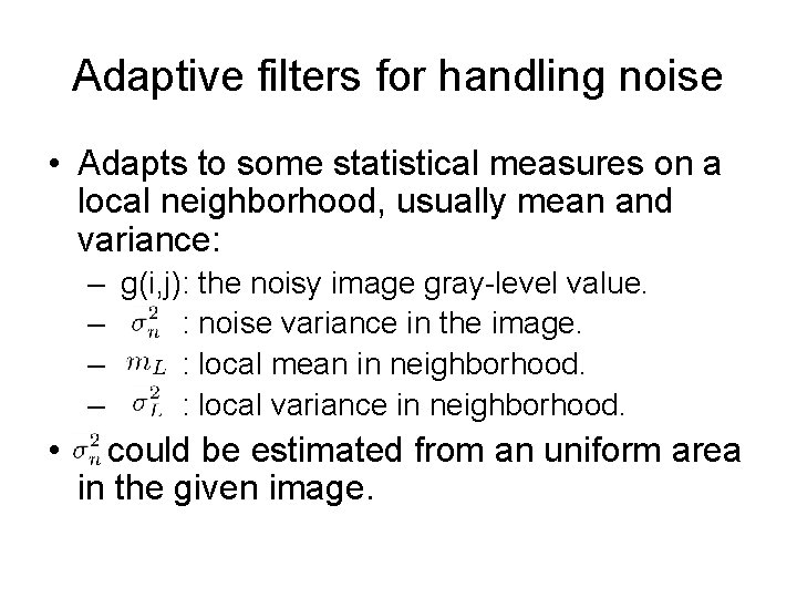
Adaptive filters for handling noise • Adapts to some statistical measures on a local neighborhood, usually mean and variance: – g(i, j): the noisy image gray-level value. – : noise variance in the image. – : local mean in neighborhood. – : local variance in neighborhood. • could be estimated from an uniform area in the given image.

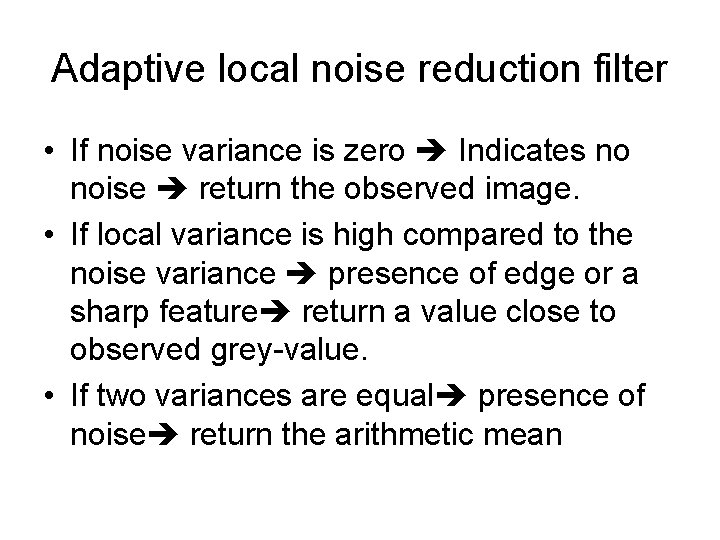
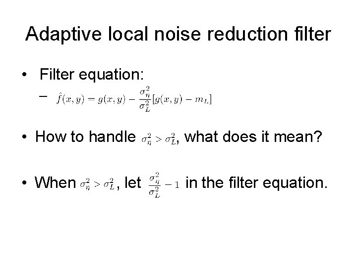
Adaptive local noise reduction filter • If noise variance is zero Indicates no noise return the observed image. • If local variance is high compared to the noise variance presence of edge or a sharp feature return a value close to observed grey-value. • If two variances are equal presence of noise return the arithmetic mean

Adaptive local noise reduction filter • Filter equation: – • How to handle • When , let , what does it mean? in the filter equation.

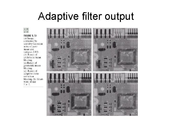
Adaptive filter output

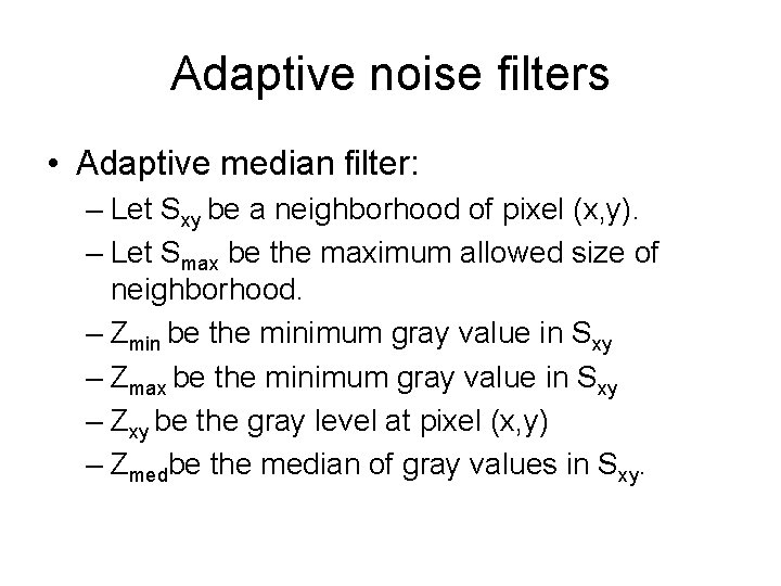
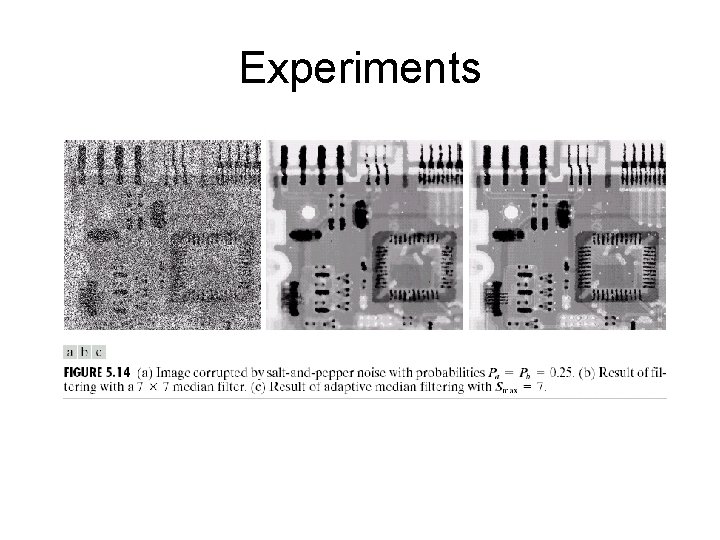
Adaptive noise filters • Adaptive median filter: – Let Sxy be a neighborhood of pixel (x, y). – Let Smax be the maximum allowed size of neighborhood. – Zmin be the minimum gray value in Sxy – Zmax be the minimum gray value in Sxy – Zxy be the gray level at pixel (x, y) – Zmedbe the median of gray values in Sxy.

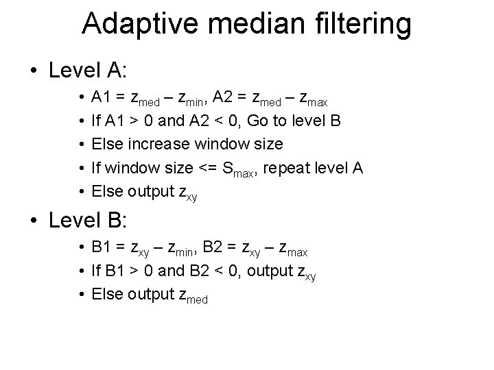
Adaptive median filtering • Level A: • • • A 1 = zmed – zmin, A 2 = zmed – zmax If A 1 > 0 and A 2 < 0, Go to level B Else increase window size If window size <= Smax, repeat level A Else output zxy • Level B: • B 1 = zxy – zmin, B 2 = zxy – zmax • If B 1 > 0 and B 2 < 0, output zxy • Else output zmed

Experiments

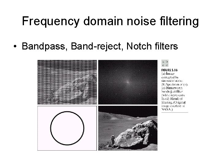
Frequency domain noise filtering • Bandpass, Band-reject, Notch filters

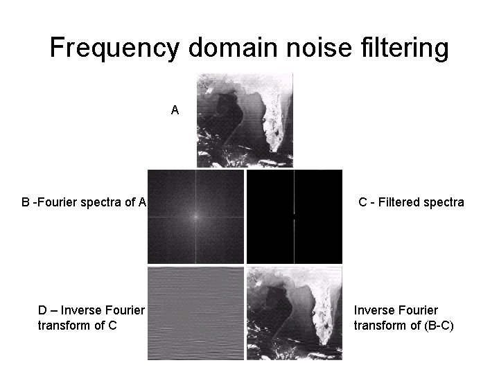
Frequency domain noise filtering A B -Fourier spectra of A D – Inverse Fourier transform of C C - Filtered spectra Inverse Fourier transform of (B-C)