Using Image Priors in Maximum Margin Classifiers Tali

Using Image Priors in Maximum Margin Classifiers Tali Brayer Margarita Osadchy Daniel Keren

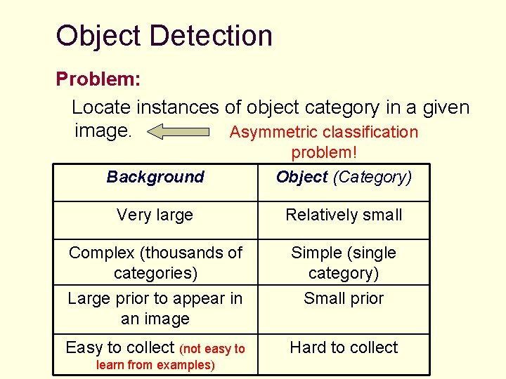
Object Detection Problem: Locate instances of object category in a given image. Asymmetric classification Background problem! Object (Category) Very large Relatively small Complex (thousands of categories) Simple (single category) Large prior to appear in an image Small prior Easy to collect (not easy to Hard to collect learn from examples)

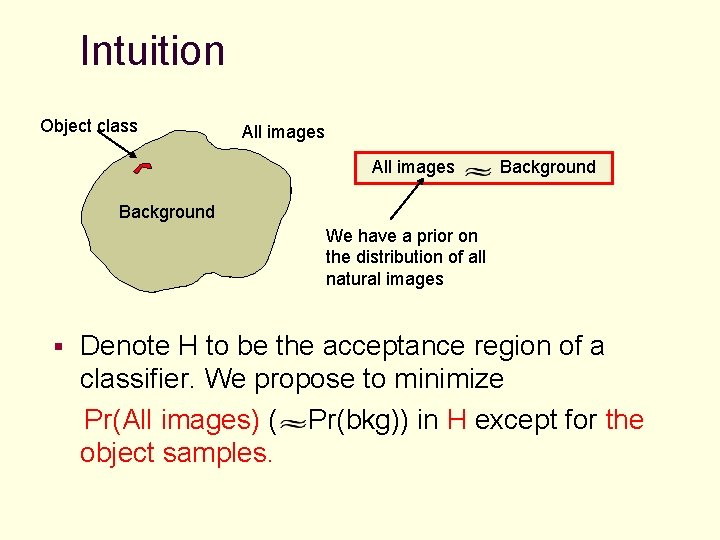
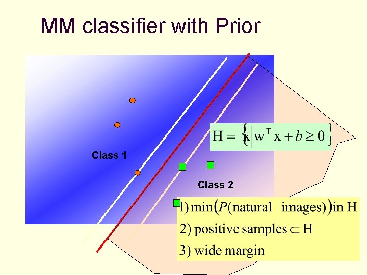
Intuition Object class All images Background We have a prior on the distribution of all natural images § Denote H to be the acceptance region of a classifier. We propose to minimize Pr(All images) ( Pr(bkg)) in H except for the object samples.

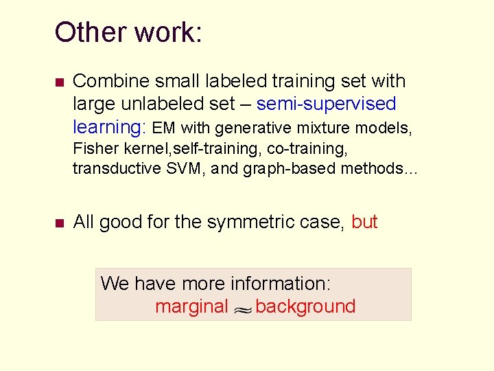
Other work: n Combine small labeled training set with large unlabeled set – semi-supervised learning: EM with generative mixture models, Fisher kernel, self-training, co-training, transductive SVM, and graph-based methods… n All good for the symmetric case, but We have more information: marginal background

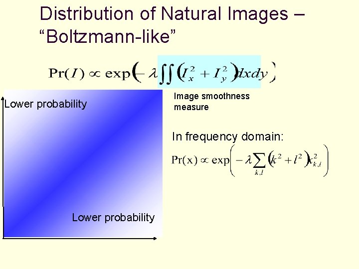
Distribution of Natural Images – “Boltzmann-like” Lower probability Image smoothness measure In frequency domain: Lower probability

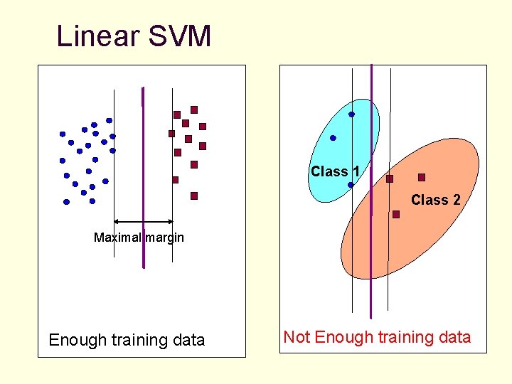
Linear SVM Class 1 Class 2 Maximal margin Enough training data Not Enough training data

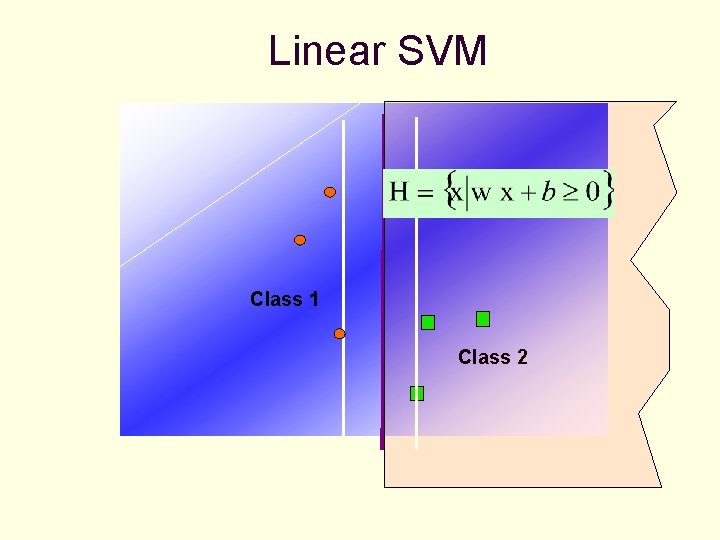
Linear SVM Class 1 Class 2

MM classifier with Prior Class 1 Class 2

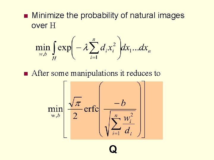
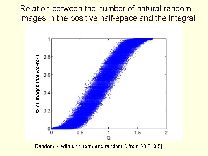
n Minimize the probability of natural images over H n After some manipulations it reduces to Q

% of images that wx+b>0 Relation between the number of natural random images in the positive half-space and the integral Random w with unit norm and random b from [-0. 5, 0. 5]

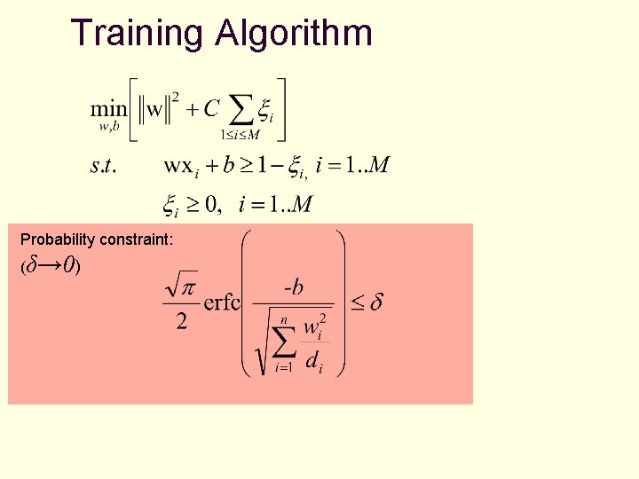
Training Algorithm Probability constraint: (δ→ 0)

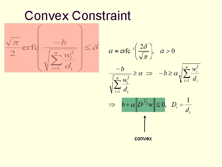
Convex Constraint convex

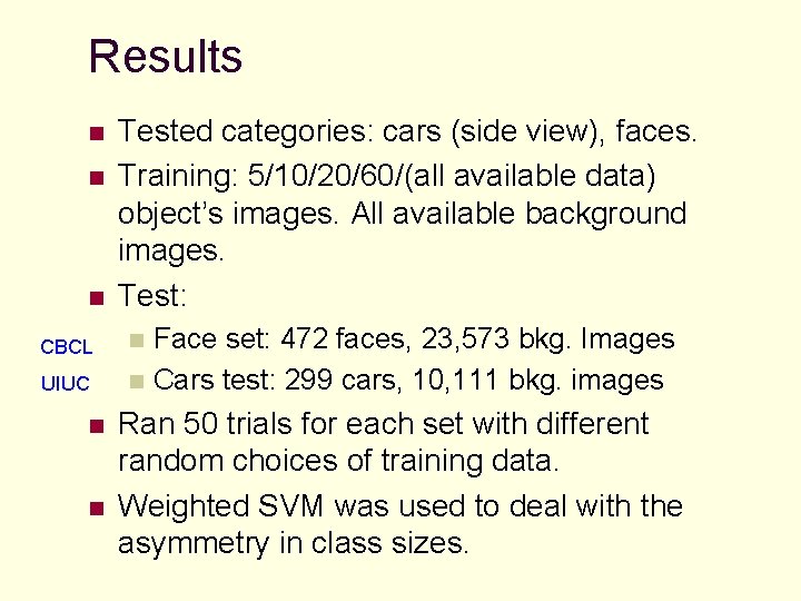
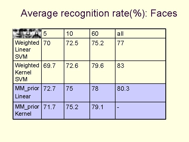
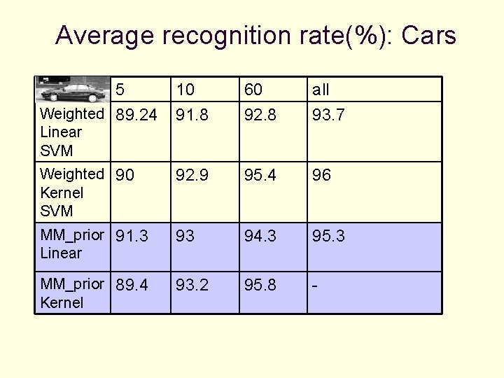
Results n n n CBCL UIUC n n Tested categories: cars (side view), faces. Training: 5/10/20/60/(all available data) object’s images. All available background images. Test: Face set: 472 faces, 23, 573 bkg. Images n Cars test: 299 cars, 10, 111 bkg. images n Ran 50 trials for each set with different random choices of training data. Weighted SVM was used to deal with the asymmetry in class sizes.

Average recognition rate(%): Faces 5 Weighted 70 10 72. 5 60 75. 2 all 77 Weighted 69. 7 Kernel SVM 72. 6 79. 6 83 MM_prior 72. 7 Linear 75 78 80. 3 MM_prior 71. 7 Kernel 75. 2 79. 1 - Linear SVM

Average recognition rate(%): Cars 5 Weighted 89. 24 10 91. 8 60 92. 8 all 93. 7 Weighted 90 Kernel SVM 92. 9 95. 4 96 MM_prior 91. 3 Linear 93 94. 3 95. 3 MM_prior 89. 4 Kernel 93. 2 95. 8 - Linear SVM

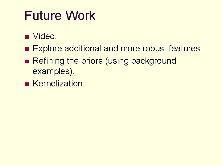
Future Work n n Video. Explore additional and more robust features. Refining the priors (using background examples). Kernelization.