Priors and conjugacy Why priors Necessary component of

Priors and conjugacy

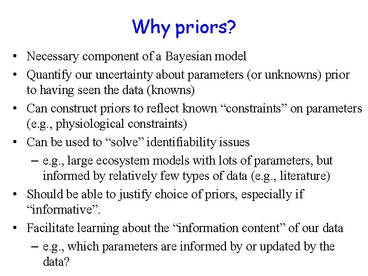
Why priors? • Necessary component of a Bayesian model • Quantify our uncertainty about parameters (or unknowns) prior to having seen the data (knowns) • Can construct priors to reflect known “constraints” on parameters (e. g. , physiological constraints) • Can be used to “solve” identifiability issues – e. g. , large ecosystem models with lots of parameters, but informed by relatively few types of data (e. g. , literature) • Should be able to justify choice of priors, especially if “informative”. • Facilitate learning about the “information content” of our data – e. g. , which parameters are informed by or updated by the data?

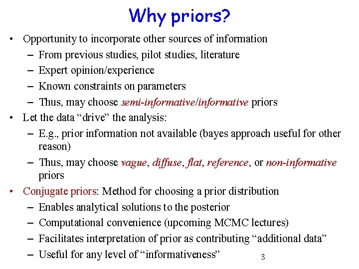
Why priors? • Opportunity to incorporate other sources of information – From previous studies, pilot studies, literature – Expert opinion/experience – Known constraints on parameters – Thus, may choose semi-informative/informative priors • Let the data “drive” the analysis: – E. g. , prior information not available (bayes approach useful for other reason) – Thus, may choose vague, diffuse, flat, reference, or non-informative priors • Conjugate priors: Method for choosing a prior distribution – Enables analytical solutions to the posterior – Computational convenience (upcoming MCMC lectures) – Facilitates interpretation of prior as contributing “additional data” – Useful for any level of “informativeness” 3

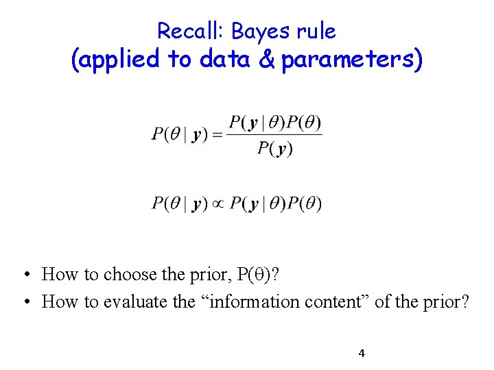
Recall: Bayes rule (applied to data & parameters) • How to choose the prior, P( )? • How to evaluate the “information content” of the prior? 4

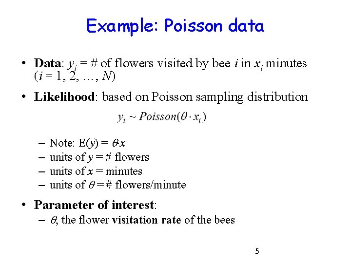
Example: Poisson data • Data: yi = # of flowers visited by bee i in xi minutes (i = 1, 2, …, N) • Likelihood: based on Poisson sampling distribution – – Note: E(y) = x units of y = # flowers units of x = minutes units of = # flowers/minute • Parameter of interest: – , the flower visitation rate of the bees 5

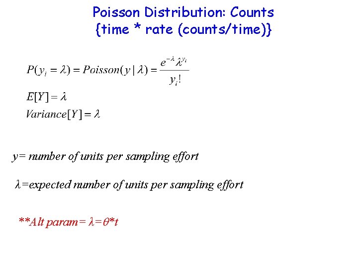
Poisson Distribution: Counts {time * rate (counts/time)} y= number of units per sampling effort λ=expected number of units per sampling effort **Alt param= λ= *t

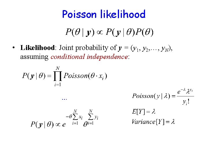
Poisson likelihood • Likelihood: Joint probability of y = (y 1, y 2, …, y. N), assuming conditional independence:

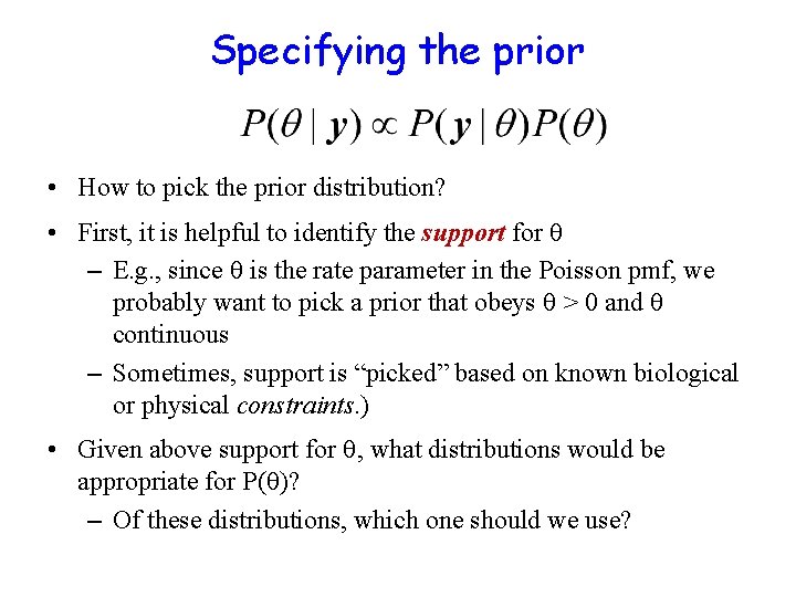
Specifying the prior • How to pick the prior distribution? • First, it is helpful to identify the support for – E. g. , since is the rate parameter in the Poisson pmf, we probably want to pick a prior that obeys > 0 and continuous – Sometimes, support is “picked” based on known biological or physical constraints. ) • Given above support for , what distributions would be appropriate for P( )? – Of these distributions, which one should we use?

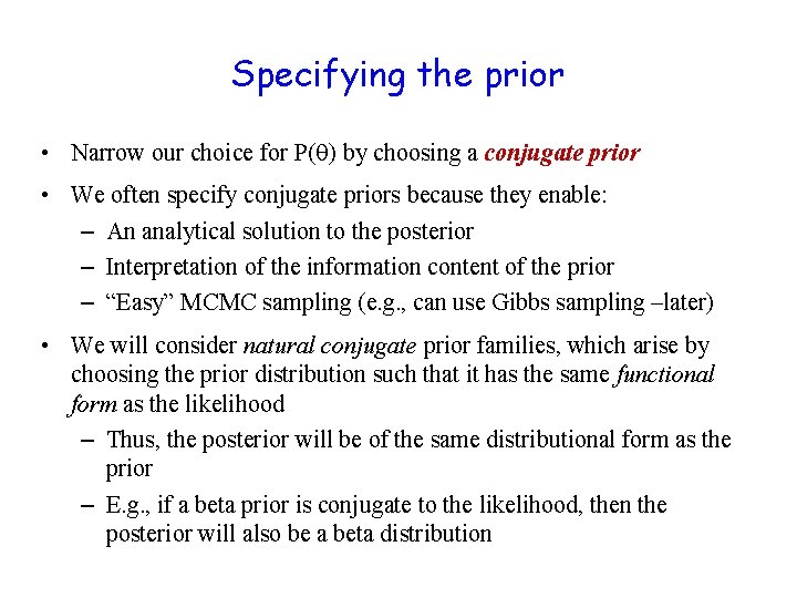
Specifying the prior • Narrow our choice for P( ) by choosing a conjugate prior • We often specify conjugate priors because they enable: – An analytical solution to the posterior – Interpretation of the information content of the prior – “Easy” MCMC sampling (e. g. , can use Gibbs sampling –later) • We will consider natural conjugate prior families, which arise by choosing the prior distribution such that it has the same functional form as the likelihood – Thus, the posterior will be of the same distributional form as the prior – E. g. , if a beta prior is conjugate to the likelihood, then the posterior will also be a beta distribution

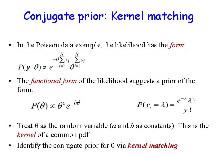
Conjugate prior: Kernel matching • In the Poisson data example, the likelihood has the form: • The functional form of the likelihood suggests a prior of the form: • Treat as the random variable (a and b as constants). This is the kernel of a common pdf • Identify the conjugate prior for via kernel matching

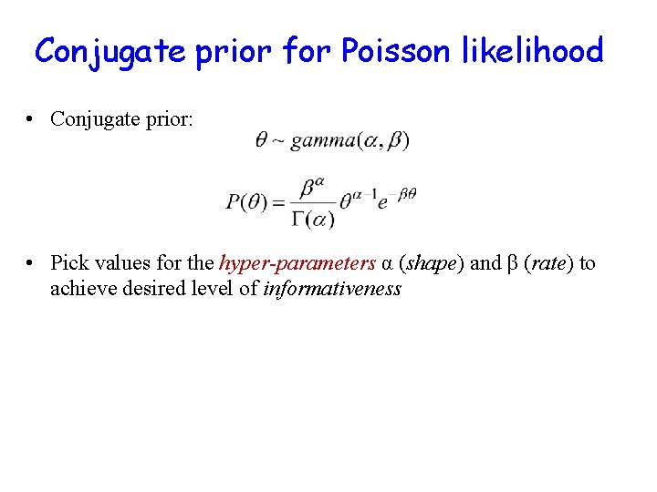
Conjugate prior for Poisson likelihood • Conjugate prior: • Pick values for the hyper-parameters α (shape) and β (rate) to achieve desired level of informativeness

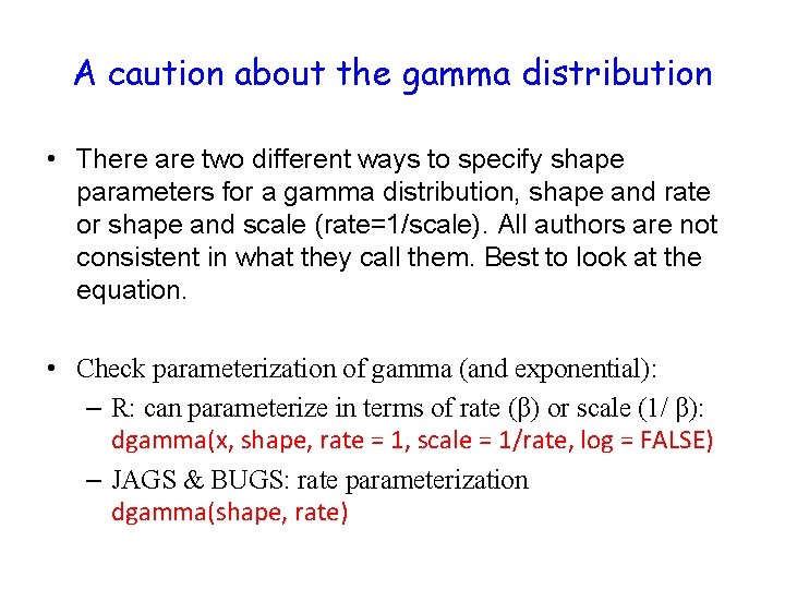
A caution about the gamma distribution • There are two different ways to specify shape parameters for a gamma distribution, shape and rate or shape and scale (rate=1/scale). All authors are not consistent in what they call them. Best to look at the equation. • Check parameterization of gamma (and exponential): – R: can parameterize in terms of rate (β) or scale (1/ β): dgamma(x, shape, rate = 1, scale = 1/rate, log = FALSE) – JAGS & BUGS: rate parameterization dgamma(shape, rate)

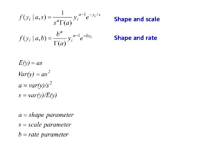
Shape and scale Shape and rate

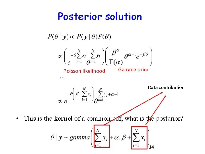
Posterior solution Poisson likelihood Gamma prior Data contribution • This is the kernel of a common pdf; what is the posterior? 14

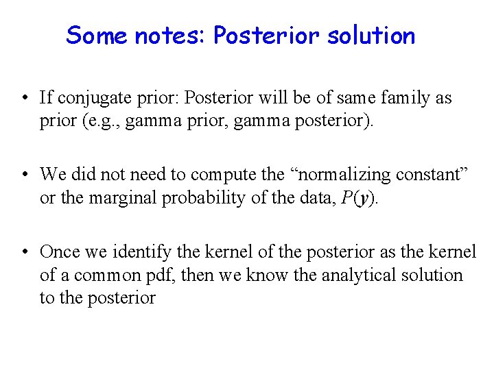
Some notes: Posterior solution • If conjugate prior: Posterior will be of same family as prior (e. g. , gamma prior, gamma posterior). • We did not need to compute the “normalizing constant” or the marginal probability of the data, P(y). • Once we identify the kernel of the posterior as the kernel of a common pdf, then we know the analytical solution to the posterior

Example 1: Poisson data with gamma prior

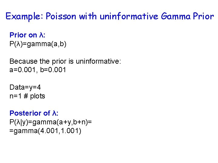
Example: Poisson with uninformative Gamma Prior • We want to estimate bee flower visitation rates in a patch. We have no prior knowledge of this rate ( ). • Based on the data y, what is P(λ|y)?

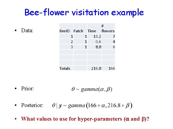
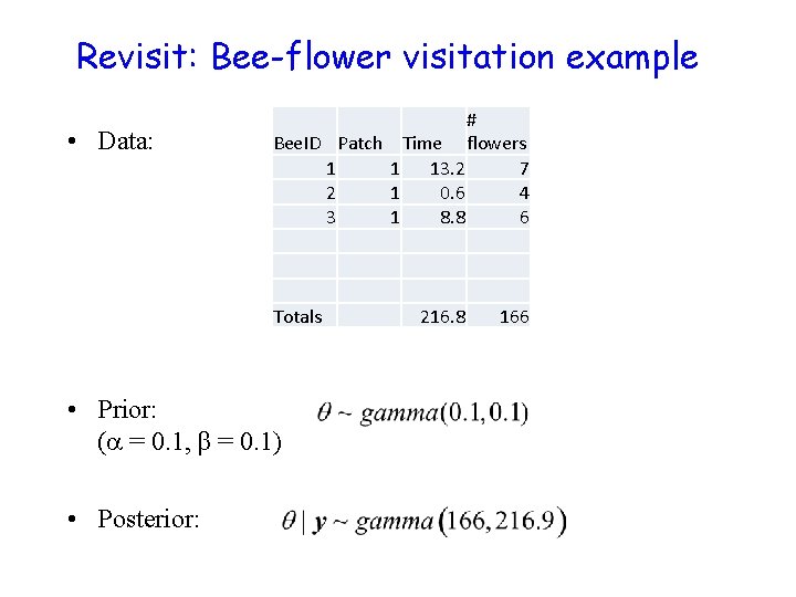
Bee-flower visitation example • Data: # Bee. ID Patch Time flowers 1 1 13. 2 7 2 1 0. 6 4 3 1 8. 8 6 Totals 216. 8 166 • Prior: • Posterior: • What values to use for hyper-parameters ( and β)?

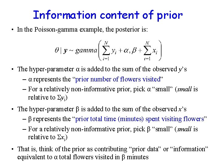
Information content of prior • In the Poisson-gamma example, the posterior is: • The hyper-parameter α is added to the sum of the observed y’s – α represents the “prior number of flowers visited” – For a relatively non-informative prior, pick α “small” (small is relative to Σyi) • The hyper-parameter β is added to the sum of the observed x’s – β represents the “prior total time (minutes) spent visiting flowers” – For a relatively non-informative prior, pick β “small” (small is relative to Σxi) • That is, think of the prior as contributing “prior data” or “information” equivalent to α total flowers visited in β minutes

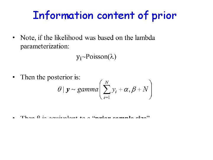
Information content of prior •

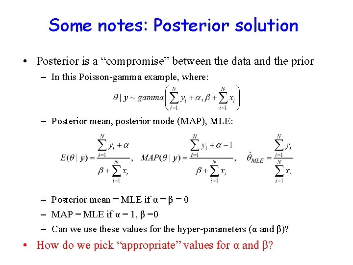
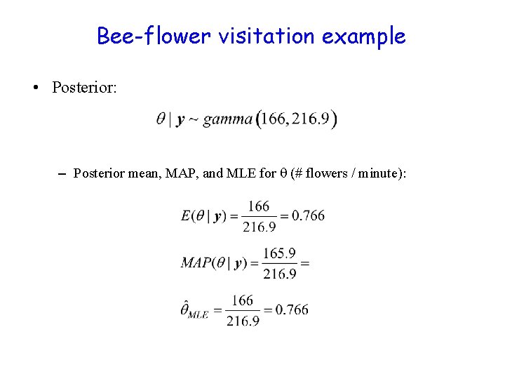
Some notes: Posterior solution • Posterior is a “compromise” between the data and the prior – In this Poisson-gamma example, where: – Posterior mean, posterior mode (MAP), MLE: – Posterior mean = MLE if α = β = 0 – MAP = MLE if α = 1, β =0 – Can we use these values for the hyper-parameters (α and β)? • How do we pick “appropriate” values for α and β?

Revisit: Bee-flower visitation example • Data: # Bee. ID Patch Time flowers 1 1 13. 2 7 2 1 0. 6 4 3 1 8. 8 6 Totals • Prior: ( = 0. 1, β = 0. 1) • Posterior: 216. 8 166

Bee-flower visitation example • Posterior: – Posterior mean, MAP, and MLE for (# flowers / minute):

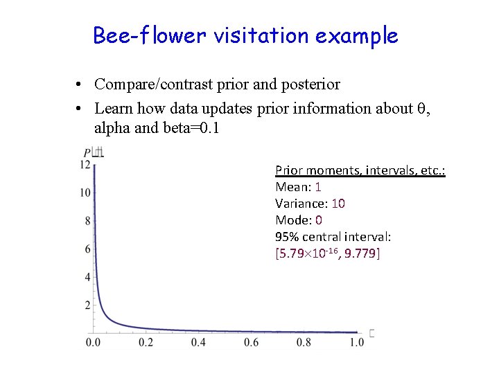
Bee-flower visitation example • Compare/contrast prior and posterior • Learn how data updates prior information about , alpha and beta=0. 1 Prior moments, intervals, etc. : Mean: 1 Variance: 10 Mode: 0 95% central interval: [5. 79 10 -16, 9. 779]

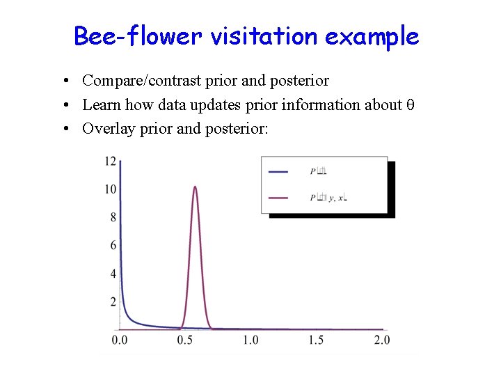
Bee-flower visitation example • Compare/contrast prior and posterior • Learn how data updates prior information about • Overlay prior and posterior:

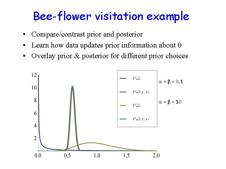
Bee-flower visitation example • Compare/contrast prior and posterior • Learn how data updates prior information about • Overlay prior & posterior for different prior choices = β = 0. 1 = β = 10

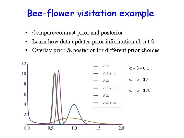
Bee-flower visitation example • Compare/contrast prior and posterior • Learn how data updates prior information about • Overlay prior & posterior for different prior choices = β = 0. 1 = β = 100

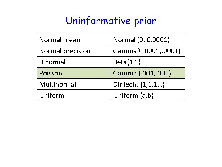
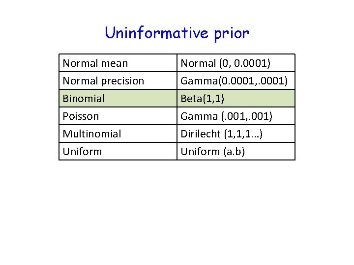
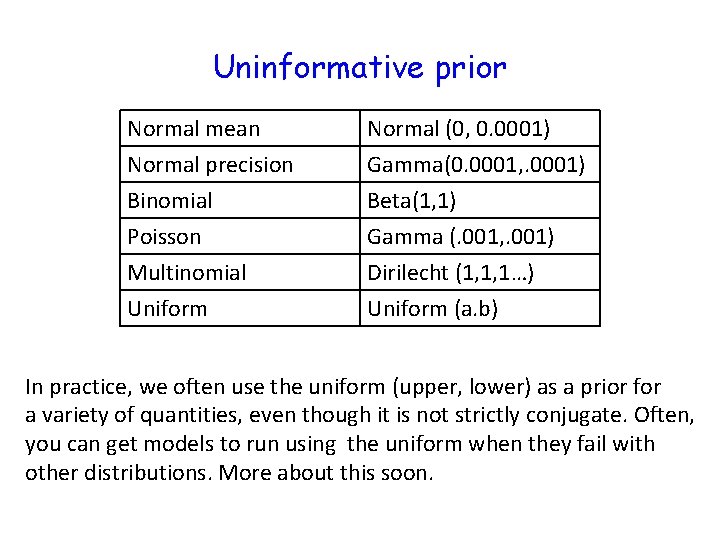
Uninformative prior Normal mean Normal precision Binomial Poisson Normal (0, 0. 0001) Gamma(0. 0001, . 0001) Beta(1, 1) Gamma (. 001, . 001) Multinomial Uniform Dirilecht (1, 1, 1…) Uniform (a. b)

Example 2 • We want to estimate the average number of rare orchid (=λ) per ha of rainforest in Costa Rica. We find 4 orchids after searching a plot 100 x 100 m. • We have no prior knowledge of the orchid density. Based on the data y, what is P(λ|y)?

Example: Poisson with uninformative Gamma Prior on λ: P(λ)=gamma(a, b) Because the prior is uninformative: a=0. 001, b=0. 001 Data=y=4 n=1 # plots Posterior of λ: P(λ|y)=gamma(a+y, b+n)= =gamma(4. 001, 1. 001)

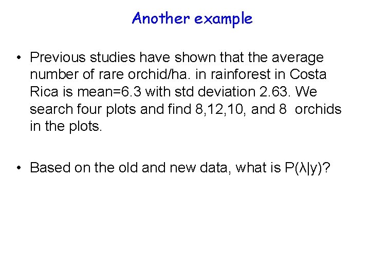
Another example • Previous studies have shown that the average number of rare orchid/ha. in rainforest in Costa Rica is mean=6. 3 with std deviation 2. 63. We search four plots and find 8, 12, 10, and 8 orchids in the plots. • Based on the old and new data, what is P(λ|y)?

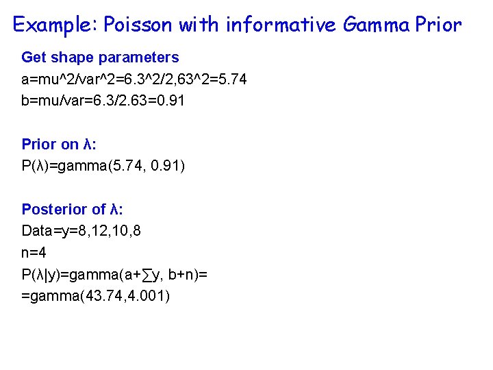
Example: Poisson with informative Gamma Prior Get shape parameters a=mu^2/var^2=6. 3^2/2, 63^2=5. 74 b=mu/var=6. 3/2. 63=0. 91 Prior on λ: P(λ)=gamma(5. 74, 0. 91) Posterior of λ: Data=y=8, 12, 10, 8 n=4 P(λ|y)=gamma(a+∑y, b+n)= =gamma(43. 74, 4. 001)

Example 2: Binomial data

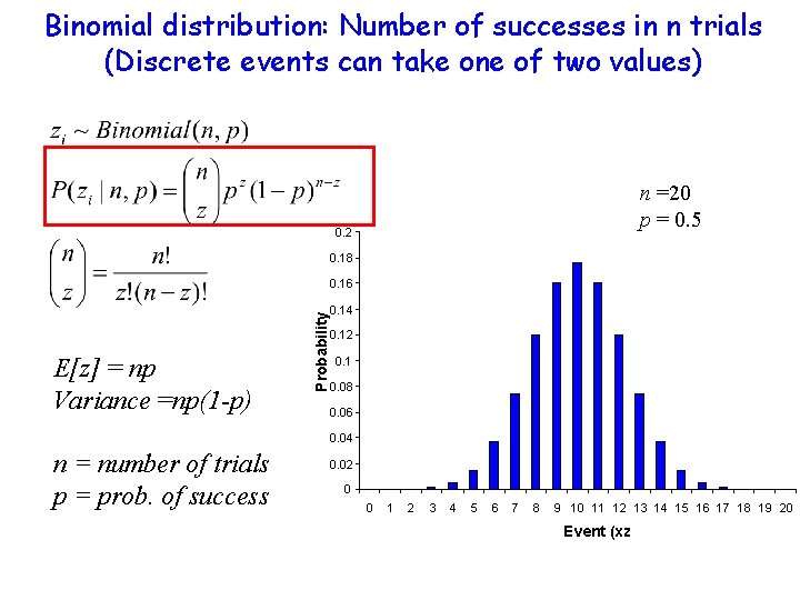
Binomial distribution: Number of successes in n trials (Discrete events can take one of two values) n =20 p = 0. 5 0. 2 0. 18 E[z] = np Variance =np(1 -p) Probability 0. 16 0. 14 0. 12 0. 1 0. 08 0. 06 0. 04 n = number of trials p = prob. of success 0. 02 0 0 1 2 3 4 5 6 7 8 9 10 11 12 13 14 15 16 17 18 19 20 Event (xz

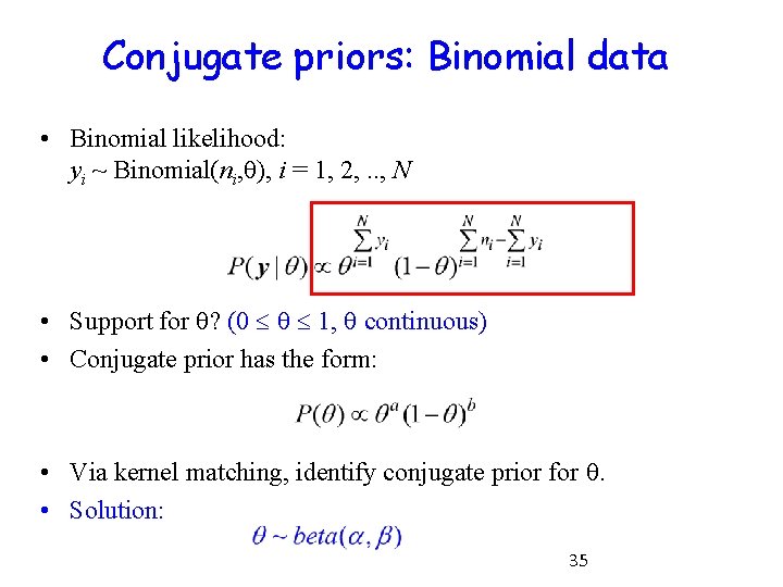
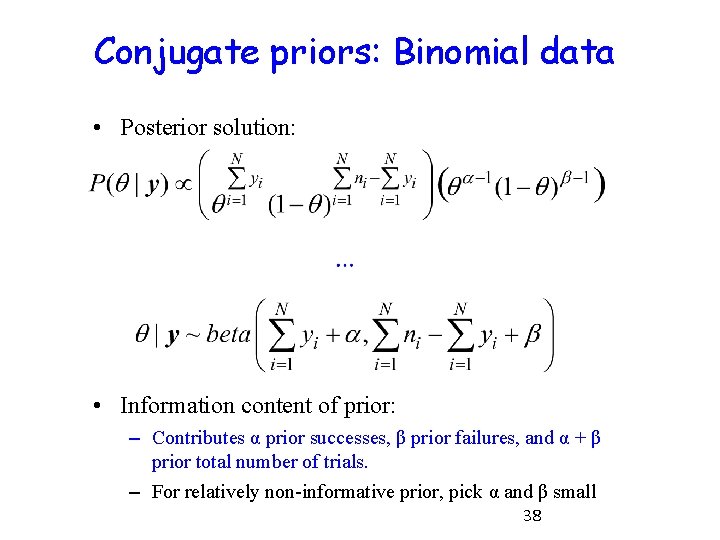
Conjugate priors: Binomial data • Binomial likelihood: yi ~ Binomial(ni, ), i = 1, 2, . . , N • Support for ? (0 1, continuous) • Conjugate prior has the form: • Via kernel matching, identify conjugate prior for . • Solution: 35

Beta distribution • Data are proportions, can take any value between 0 and 1. • The data arise through any process that produces continuous data between 0 and 1. For example, a distribution of survival probability or the proportion of landscape that has been invaded by an exotic. • Different from the binomial which predicts number of survivors conditioned on the survival probability.

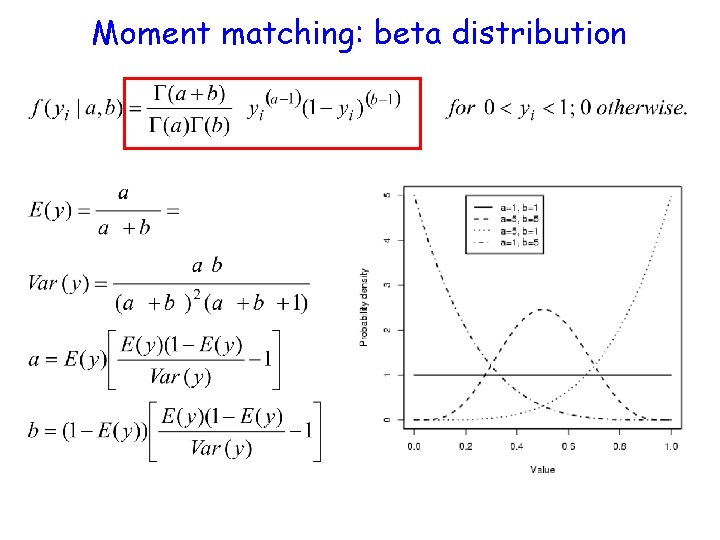
Moment matching: beta distribution

Conjugate priors: Binomial data • Posterior solution: • Information content of prior: – Contributes α prior successes, β prior failures, and α + β prior total number of trials. – For relatively non-informative prior, pick α and β small 38

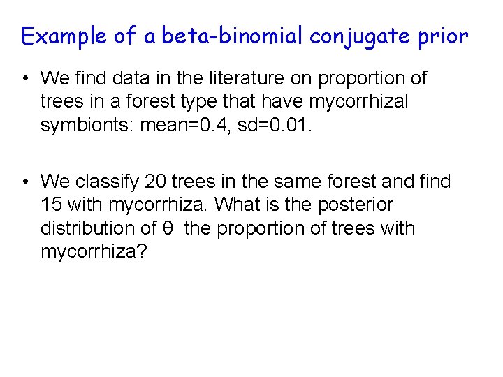
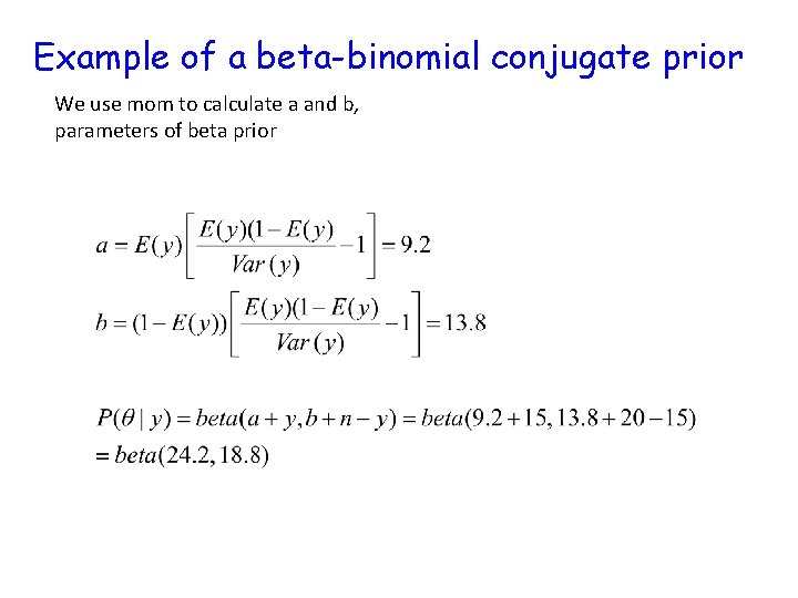
Example of a beta-binomial conjugate prior • We find data in the literature on proportion of trees in a forest type that have mycorrhizal symbionts: mean=0. 4, sd=0. 01. • We classify 20 trees in the same forest and find 15 with mycorrhiza. What is the posterior distribution of θ the proportion of trees with mycorrhiza?

Example of a beta-binomial conjugate prior We use mom to calculate a and b, parameters of beta prior

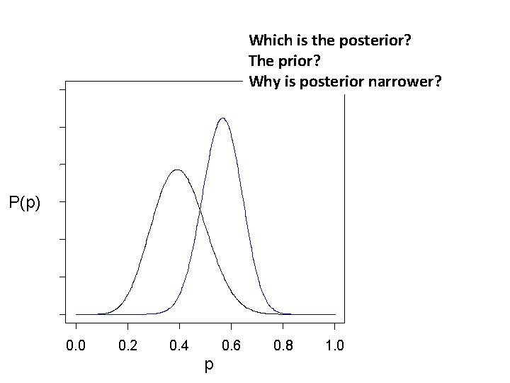
Which is the posterior? The prior? Why is posterior narrower? P(p) 0. 0 0. 2 0. 4 0. 6 p 0. 8 1. 0

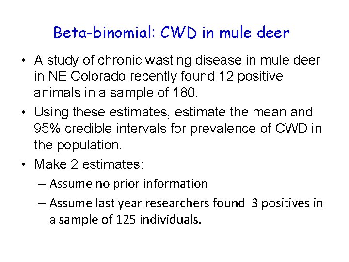
Beta-binomial: CWD in mule deer • A study of chronic wasting disease in mule deer in NE Colorado recently found 12 positive animals in a sample of 180. • Using these estimates, estimate the mean and 95% credible intervals for prevalence of CWD in the population. • Make 2 estimates: – Assume no prior information – Assume last year researchers found 3 positives in a sample of 125 individuals.

Uninformative prior Normal mean Normal precision Binomial Poisson Normal (0, 0. 0001) Gamma(0. 0001, . 0001) Beta(1, 1) Gamma (. 001, . 001) Multinomial Uniform Dirilecht (1, 1, 1…) Uniform (a. b)

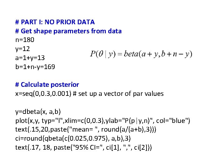
# PART I: NO PRIOR DATA # Get shape parameters from data n=180 y=12 a=1+y=13 b=1+n-y=169 # Calculate posterior x=seq(0, 0. 3, 0. 001) # set up a vector of par values y=dbeta(x, a, b) plot(x, y, typ="l", xlim=c(0, 0. 3), ylab="P(p|y, n)", col="blue") text(. 15, 20, paste("mean= ", round(a/(a+b), 3))) ci=round(qbeta(c(0. 025, 0. 975), a, b), 3) text(. 17, 18, paste("95% CI=", ci[1], ", ", ci[2]))

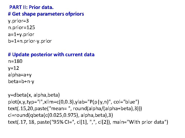
PART II: Prior data. # Get shape parameters ofpriors y. prior=3 n. prior=125 a=1+y. prior b=1+n. prior-y. prior # Update posterior with current data n=180 y=12 alpha=a+y beta=b+n-y y=dbeta(x, alpha, beta) plot(x, y, typ="l", xlim=c(0, 0. 3), ylab="P(p|y, n)", col="blue") text(. 15, 20, paste("mean= ", round(alpha/(alpha+beta), 3))) ci=round(qbeta(c(0. 025, 0. 975), alpha, beta), 3) text(. 17, 18, paste("95% CI=", ci[1], ", ", ci[2]), main="With prior data")

Other distributions

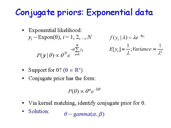
Conjugate priors: Exponential data • Exponential likelihood: yi ~ Expon( ), i = 1, 2, . . , N • Support for ? ( R+) • Conjugate prior has the form: • Via kernel matching, identify conjugate prior for . • Solution:

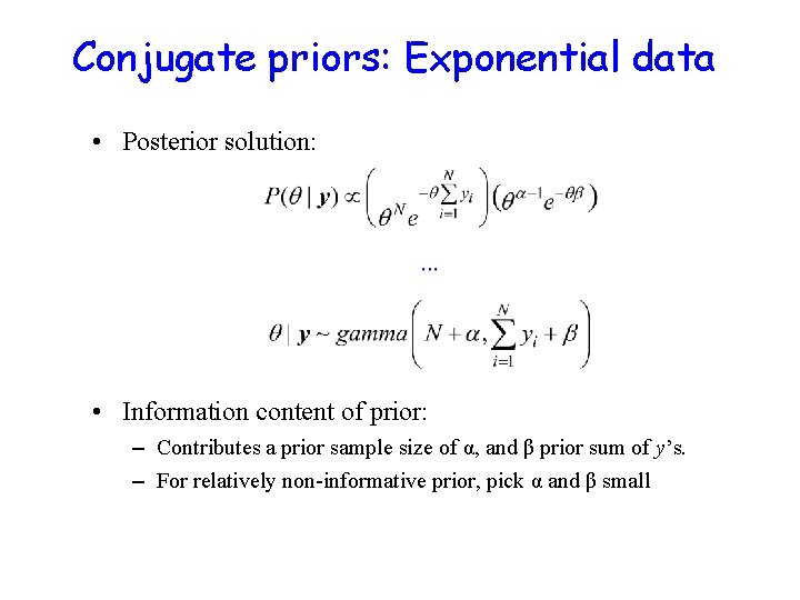
Conjugate priors: Exponential data • Posterior solution: • Information content of prior: – Contributes a prior sample size of α, and β prior sum of y’s. – For relatively non-informative prior, pick α and β small

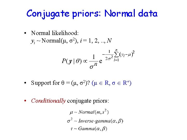
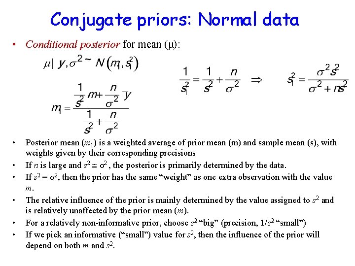
Conjugate priors: Normal data • Normal likelihood: yi ~ Normal(μ, σ2), i = 1, 2, . . , N • Support for = (μ, σ2)? (μ R, σ R+) • Conditionally conjugate priors:

Conjugate priors: Normal data • Conditional posterior for mean (μ): • • • Posterior mean (m 1) is a weighted average of prior mean (m) and sample mean (s), with weights given by their corresponding precisions If n is large and s 2 σ2 , the posterior is primarily determined by the data. If s 2 = σ2, then the prior has the same “weight” as one extra observation with the value m. The relative influence of the prior is mainly determined by the value assigned to s 2 and is relatively unaffected by the prior mean (m). For a relatively non-informative prior, choose s 2 “big” (precision, 1/s 2 “small”) If we pick an informative (“small”) value for s 2, then the influence of the prior will depend on both m and s 2.

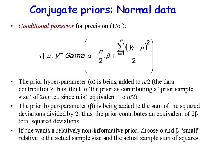
Conjugate priors: Normal data • Conditional posterior for precision (1/σ2): • The prior hyper-parameter (α) is being added to n/2 (the data contribution); thus, think of the prior as contributing a “prior sample size” of 2α (i. e. , since α is “equivalent” to n/2) • The prior hyper-parameter (β) is being added to the sum of the squared deviations divided by 2; thus, the prior contributes an equivalent of 2β total squared deviations. • If one wants a relatively non-informative prior, choose α and β “small” relative to the actual sample size and the actual sample sum of squares.

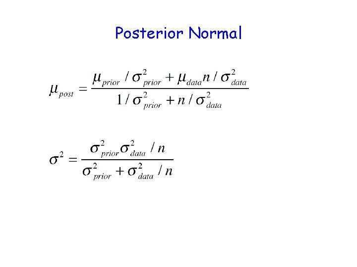
Posterior Normal

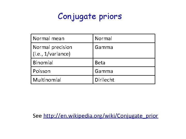
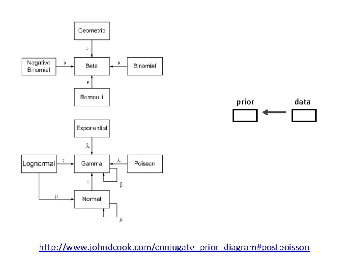
Conjugate priors Normal mean Normal precision (i. e. , 1/variance) Gamma Binomial Beta Poisson Gamma Multinomial Dirilecht See http: //en. wikipedia. org/wiki/Conjugate_prior

prior data http: //www. johndcook. com/conjugate_prior_diagram#postpoisson

Conjugate priors: Summary • See distribution hand-out for other examples of likelihoodconjugate prior relationships – E. g. , Multinomial data + Dirichlet conjugate prior • Note: we are NOT restricted to using conjugate priors, but their use facilitates: – Interpretation of information content to prior – Analytical solutions to conditional posteriors – Selection and development of MCMC sampling routines • If we don’t use conjugate priors, need to consider: – The support of , or it’s components (multi-parameter models) – How to select relatively non-informative priors (e. g. , “rulesof-thumb” for conjugate priors may still apply, such as pick α “small”)

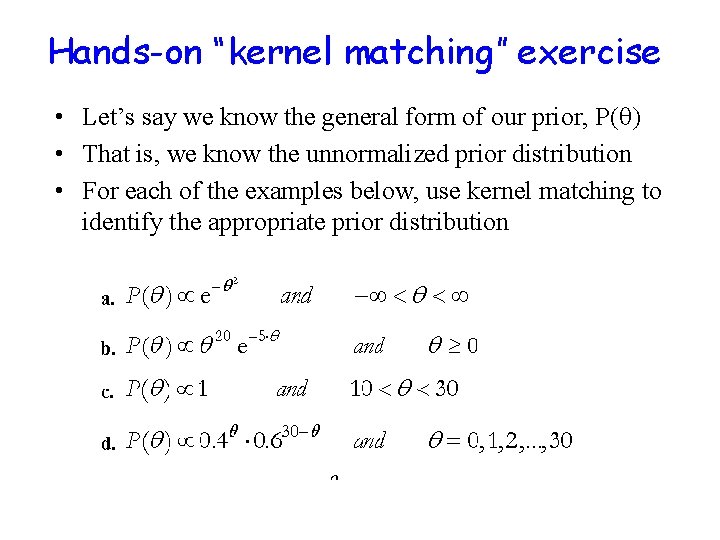
Hands-on “kernel matching” exercise • Let’s say we know the general form of our prior, P( ) • That is, we know the unnormalized prior distribution • For each of the examples below, use kernel matching to identify the appropriate prior distribution

Priors: additional considerations • Proper vs improper priors • Improper prior may lead to improper posterior • Flat priors for parameters with unbounded support (e. g. , R) • Alternatively, chose ~ U(A, B) • Non-informative priors • Nearly impossible to specify a truly non-informative prior (often results in improper prior) • Having a “flat” shape doesn’t always mean a prior is more noninformative; interpretation of prior as contributing prior information is more appropriate (when able to do) • Besides conjugacy and a couple other techniques, there isn’t a clear “recipe” for choosing a particular prior distribution • If the likelihood truly dominates the posterior, then the actual form of the prior shouldn’t matter much • Evaluate the sensitivity of the posterior to the prior specification

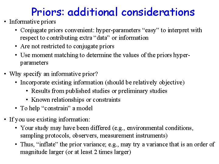
Priors: additional considerations • Informative priors • Conjugate priors convenient: hyper-parameters “easy” to interpret with respect to contributing extra “data” or information • Are not restricted to conjugate priors • Use moment matching to determine the values of the priors hyperparameters • Why specify an informative prior? • Incorporate existing information (should be relatively objective) • Results from published studies or preliminary studies • Known relationships or constraints • To help “constrain” a model • If you use existing information: • Your study may have been differed (e. g. , environmental conditions, sampling protocols, observers, measurement instruments) • Thus, “inflate” the prior variance; e. g. , may try a variance that is an order of magnitude larger (or at least 2 times larger)

Uninformative prior Normal mean Normal precision Binomial Poisson Normal (0, 0. 0001) Gamma(0. 0001, . 0001) Beta(1, 1) Gamma (. 001, . 001) Multinomial Uniform Dirilecht (1, 1, 1…) Uniform (a. b) In practice, we often use the uniform (upper, lower) as a prior for a variety of quantities, even though it is not strictly conjugate. Often, you can get models to run using the uniform when they fail with other distributions. More about this soon.

References / further reading • Gelman, Carlin, Stern, Rubin (2004) Bayesian Data Analysis. Chapman & Hall/CRC. • Discussion of priors, conjugate priors, and information content of priors (e. g. , Chapter 2) • Multiple examples for different likelihood models. • Wikipedia table of likelihood-conjugate prior relationships: http: //en. wikipedia. org/wiki/Conjugate_prior