Frequency Response Analysis 1 Frequency Response Analysis In

Frequency Response Analysis 1

Frequency Response Analysis • In steady state, sinusoidal inputs to a linear system generate sinusoidal responses of the same frequency. Sine in sine out • However, both amplitude and phase shift angle of input and output are different. • These differences are functions of frequency. • In frequency response analysis, the frequency of the input signal is varied over a certain range and the resulting response is studied. 2

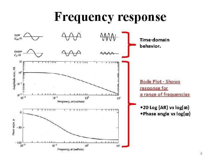
Frequency response Time-domain behavior. Bode Plot - Shows response for a range of frequencies • 20 Log (AR) vs log( ) • Phase angle vs log( ) 3

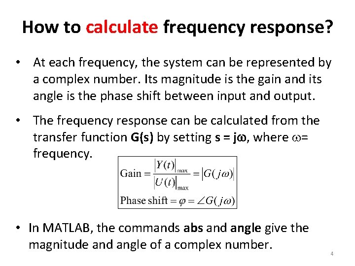
How to calculate frequency response? • At each frequency, the system can be represented by a complex number. Its magnitude is the gain and its angle is the phase shift between input and output. • The frequency response can be calculated from the transfer function G(s) by setting s = j , where = frequency. • In MATLAB, the commands abs and angle give the magnitude and angle of a complex number. 4

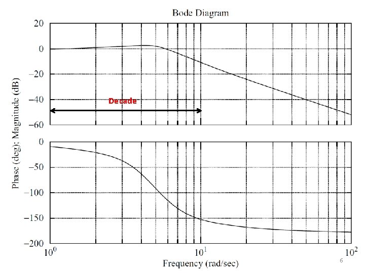
Frequency Domain Plots: Bode Plot A Bode diagram consists of two graphs: – One is a plot of the logarithm of the magnitude of a sinusoidal transfer function. – The other is a plot of the phase angle. – Both are plotted against the frequency on a logarithmic scale. 5

Decade 6

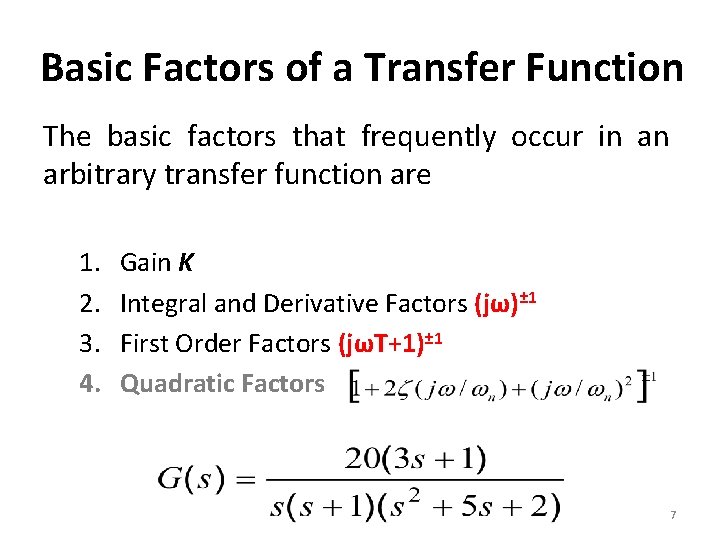
Basic Factors of a Transfer Function The basic factors that frequently occur in an arbitrary transfer function are 1. 2. 3. 4. Gain K Integral and Derivative Factors (jω)± 1 First Order Factors (jωT+1)± 1 Quadratic Factors 7

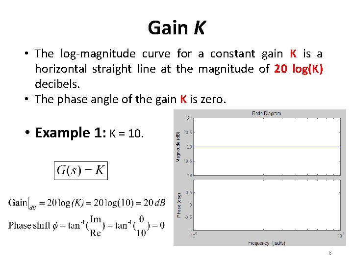
Gain K • The log-magnitude curve for a constant gain K is a horizontal straight line at the magnitude of 20 log(K) decibels. • The phase angle of the gain K is zero. • Example 1: K = 10. 8

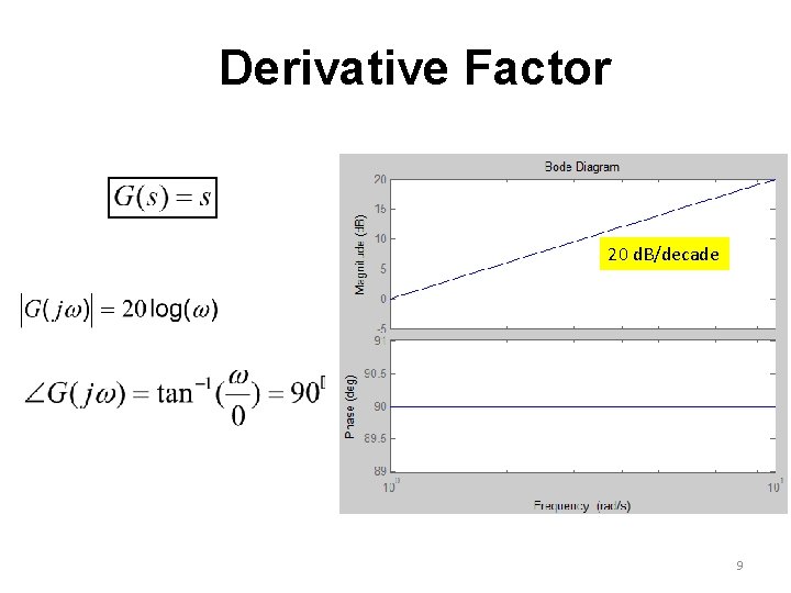
Derivative Factor 20 d. B/decade 9

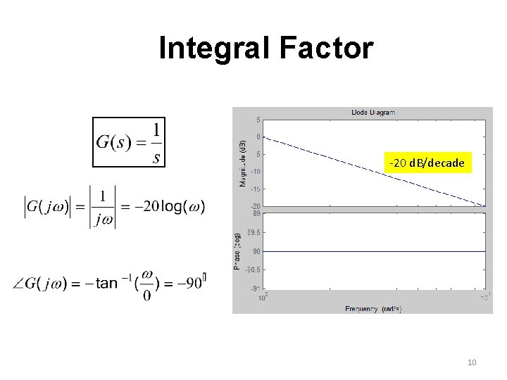
Integral Factor -20 d. B/decade 10

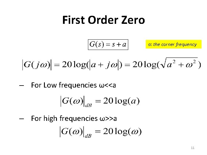
First Order Zero a: the corner frequency – For Low frequencies ω<<a – For high frequencies ω>>a 11

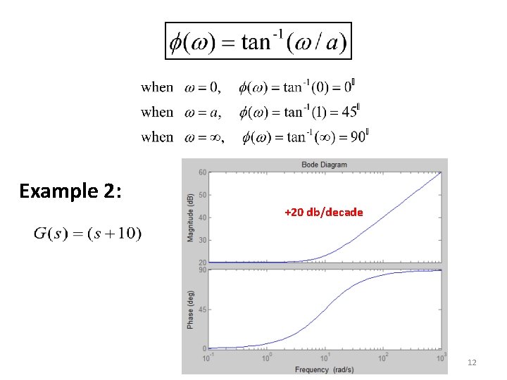
Example 2: +20 db/decade 12

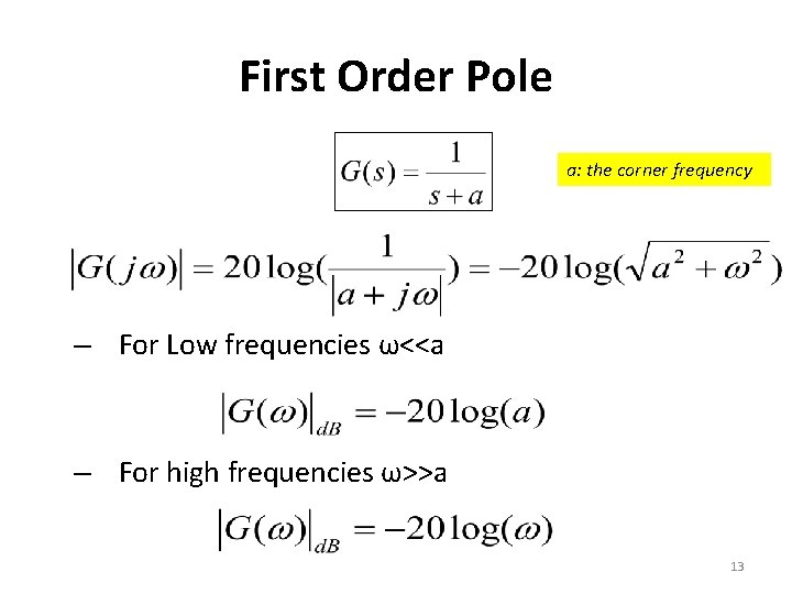
First Order Pole a: the corner frequency – For Low frequencies ω<<a – For high frequencies ω>>a 13

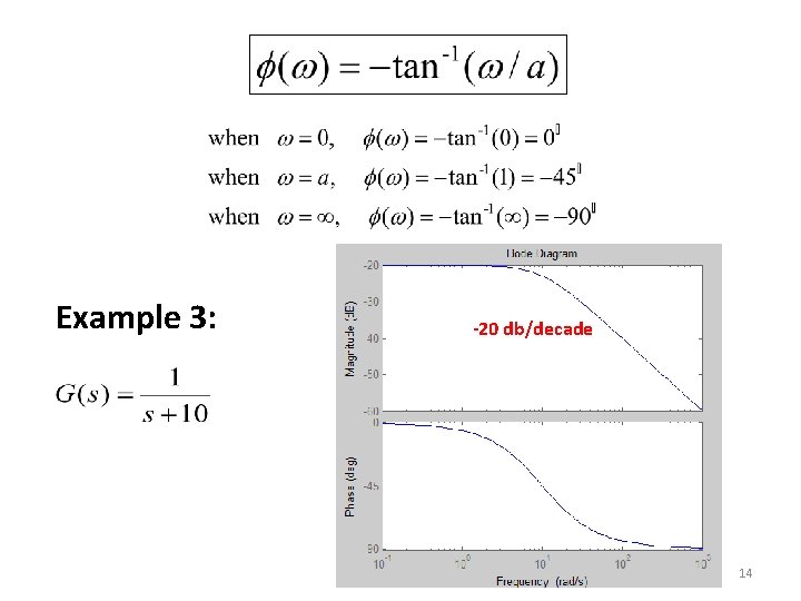
Example 3: -20 db/decade 14

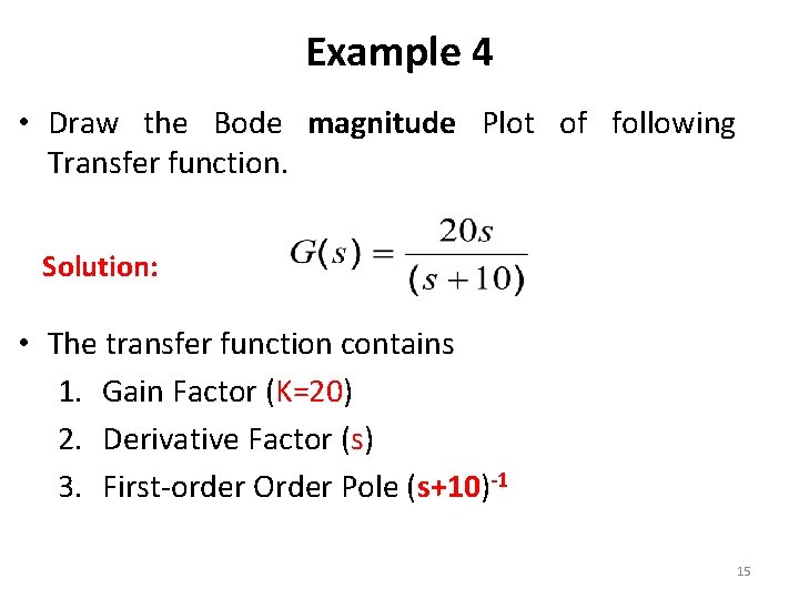
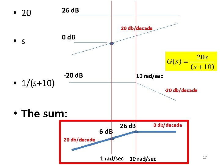
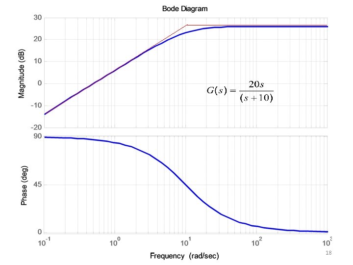
Example 4 • Draw the Bode magnitude Plot of following Transfer function. Solution: • The transfer function contains 1. Gain Factor (K=20) 2. Derivative Factor (s) 3. First-order Order Pole (s+10)-1 15

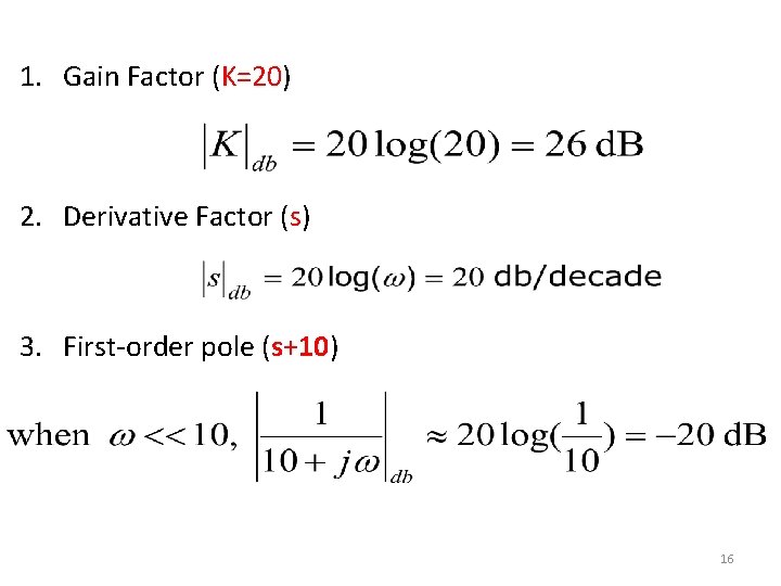
1. Gain Factor (K=20) 2. Derivative Factor (s) 3. First-order pole (s+10) 16

• 20 26 d. B 20 db/decade • s • 1/(s+10) 0 d. B -20 d. B 10 rad/sec -20 db/decade • The sum: 6 d. B 26 d. B 0 db/decade 20 db/decade 1 rad/sec 10 rad/sec 17

18

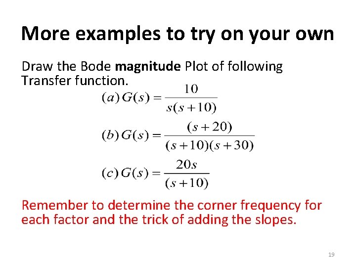
More examples to try on your own Draw the Bode magnitude Plot of following Transfer function. Remember to determine the corner frequency for each factor and the trick of adding the slopes. 19

Bode plot and relative stability • As we have seen before, root locus can be used to design compensators. Bode plot is another important tool which can be used for this purpose. • However, what we are interested in now is to use Bode plot to determine the relative stability of a given system. • Remember that two systems may be stable, but one is more stable than the other. 20

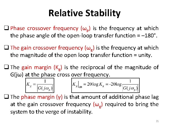
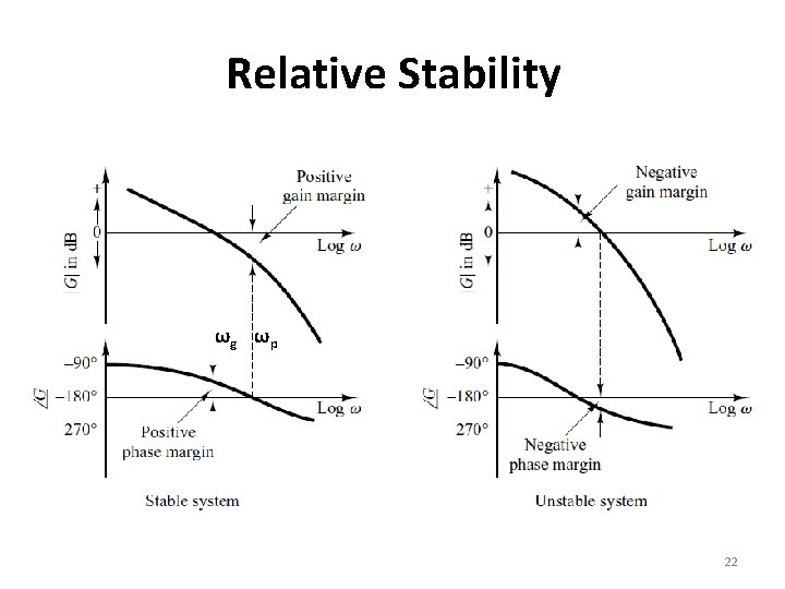
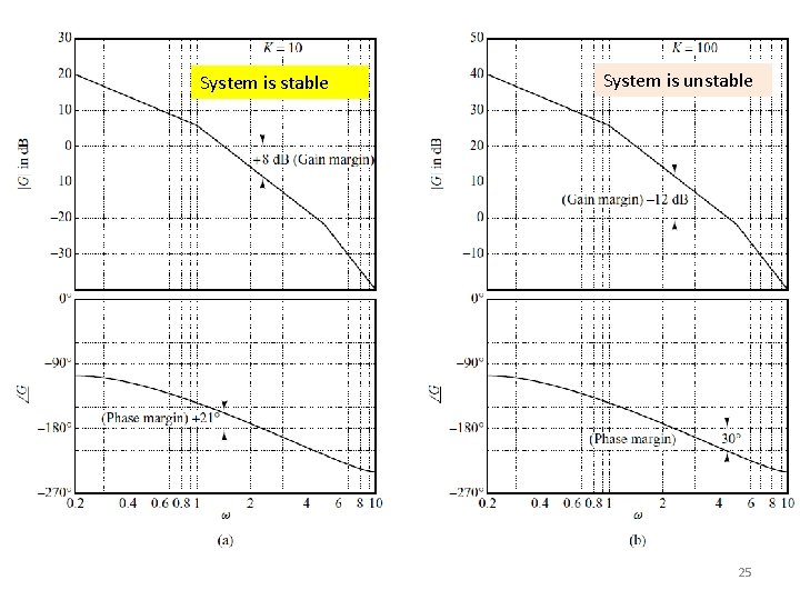
Relative Stability q Phase crossover frequency (ωp) is the frequency at which the phase angle of the open-loop transfer function = – 180°. q The gain crossover frequency (ωg) is the frequency at which the magnitude of the open loop transfer function = unity. q The gain margin (Kg) is the reciprocal of the magnitude of G(jω) at the phase cross over frequency. q The phase margin (γ) is that amount of additional phase lag at the gain crossover frequency (ωg) required to bring the system to the verge of instability. 21

Relative Stability ωg ωp 22

Relative Stability • The higher the gain margin and phase margin, the more stable is the system. • If the gain margin or phase margin are negative, the system is unstable. 23

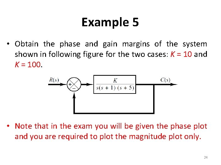
Example 5 • Obtain the phase and gain margins of the system shown in following figure for the two cases: K = 10 and K = 100. • Note that in the exam you will be given the phase plot and you are required to plot the magnitude plot only. 24

System is stable System is unstable 25