Open vs Closed Loop Frequency Response And Frequency

 Goal: 1) Define")


 Gp(s) From specs: => desired Bode shape of Gol(s)")
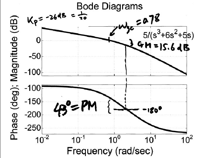

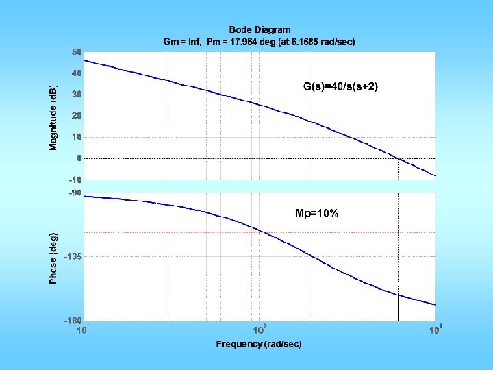
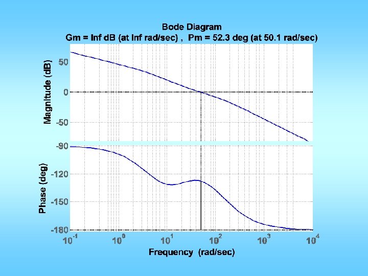
![clear all; n=[0 0 40]; d=[1 2 0]; figure(1); clf; margin(n, d); %proportional control](https://slidetodoc.com/presentation_image_h2/aa76c690e6edadf930086ad607ce16c3/image-28.jpg "clear all; n=[0 0 40]; d=[1 2 0]; figure(1); clf; margin(n, d); %proportional control")

 Goal: select z and p so that max phase lead")

![Lead design example • Plant transfer function is given by: • n=[50000]; d=[1 60](https://slidetodoc.com/presentation_image_h2/aa76c690e6edadf930086ad607ce16c3/image-37.jpg "Lead design example • Plant transfer function is given by: • n=[50000]; d=[1 60")
![n=[50000]; d=[1 60 500 0]; G=tf(n, d); figure(1); margin(G); Mp_d = 16/100; zeta_d =0.](https://slidetodoc.com/presentation_image_h2/aa76c690e6edadf930086ad607ce16c3/image-38.jpg "n=[50000]; d=[1 60 500 0]; G=tf(n, d); figure(1); margin(G); Mp_d = 16/100; zeta_d =0.")

; Magnitude plot shifted up 3 So, gc")
![n=[50]; d=[1/5 1 0]; figure(1); clf; margin(n, d); grid; hold on; Mp = 20/100;](https://slidetodoc.com/presentation_image_h2/aa76c690e6edadf930086ad607ce16c3/image-42.jpg "n=[50]; d=[1/5 1 0]; figure(1); clf; margin(n, d); grid; hold on; Mp = 20/100;")

![n=[50]; d=[1/5 1 0]; figure(1); clf; margin(n, d); grid; hold on; Mp = 20/100;](https://slidetodoc.com/presentation_image_h2/aa76c690e6edadf930086ad607ce16c3/image-49.jpg "n=[50]; d=[1/5 1 0]; figure(1); clf; margin(n, d); grid; hold on; Mp = 20/100;")
- Slides: 55
Open vs Closed Loop Frequency Response And Frequency Domain Specifications C(s) Goal: 1) Define typical “good” frequency response shape for closed-loop 2) Relate closed-loop freq response shape to step response shape 3) Relate closed-loop freq shape to open-loop freq response shape 4) Design C(s) to make C(s)G(s) into “good” shape.
Mr and BW are widely used Closed-loop phase resp. rarely used
Prototype 2 nd order system closed-loop frequency response No resonance for z <= 0. 7 Mr=0. 3 d. B for z=0. 6 z=0. 1 Mr=1. 2 d. B for z=0. 5 0. 2 For small zeta, resonance freq is about wn 0. 3 Mr=2. 6 d. B for z=0. 4 BW ranges from 0. 5 wn to 1. 5 wn For good z range, BW is 0. 8~1. 25 wn -3 d. B BW 0. 63 So take BW ≈ wn 1. 58 0. 79 1. 26 w/wn
Closed-loop BW to wn ratio BW≈wn z
Prototype 2 nd order system closed-loop frequency response z=0. 1 When z >=0. 6 no visible resonance peak 0. 2 0. 3 When z <=0. 5 visible resonance peak near w=wn Since we design for z >=0. 5, Mr and wr are of less value No resonance for z <= 0. 7 Mr<0. 5 d. B for z=0. 6 Mr=1. 2 d. B for z=0. 5 Mr=2. 6 d. B for z=0. 4 w=wn w/wn
Prototype 2 nd order system closed-loop frequency response Mr vs z
Mr in d. B
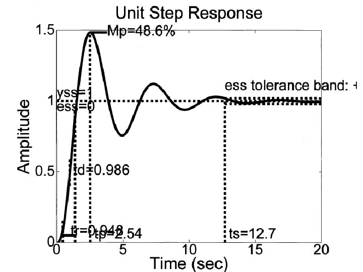
Percentage Overshoot in closed-loop step response z > 0. 5 is good z
Percentage Overshoot in closed-loop step response Mr < 15% is good, >40% not tolerable Mr
Percentage Overshoot in closed-loop step response Mr < 1 d. B is good, >3 d. B not tolerable Mr in d. B
z=0. 1 0. 2 0. 3 0. 4 Open loop frequency response wgc In the range of good zeta, wgc is about 0. 7 times wn w/wn
Open-loop wgc to wn ratio wgc≈0. 7 wn z
z=0. 1 In the range of good zeta, PM is about 100*z 0. 2 0. 3 0. 4 w/wn
Phase Margin PM = 100 z z
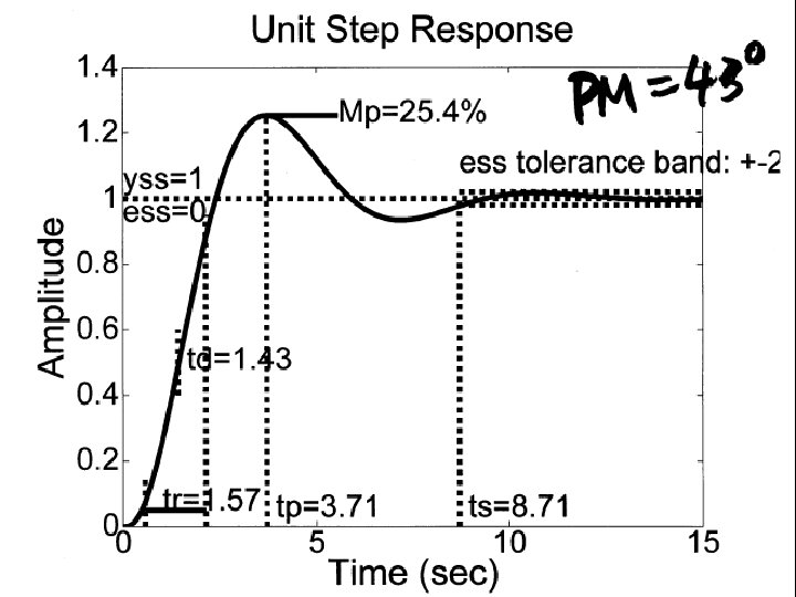
Percentage overshoot: Mp PM+Mp =70 line Percentage Overshoot in closed-loop step response Phase Margin in degrees: PM in deg
Important relationships • Closed-loop BW are very close to wn • Open-loop gain cross over wgc ≈ (0. 65~0. 8)* wn, • When z <= 0. 6, wr and wn are close • When z >= 0. 7, no resonance • z determines phase margin and Mp: z PM Mp 0. 4 0. 5 0. 6 0. 7 44 53 61 25 16 10 PM+Mp ≈70 67 5 deg % ≈100 z
Desired Bode plot shape High low-freq-gain for steady state tracking Low high-freq-gain for noise attenuation Sufficient PM near wgc for stability wgc w 0 d. B 0 -90 -180 w
Controller design with Bode C(s) Gp(s) From specs: => desired Bode shape of Gol(s) Make Bode plot of Gp(s) Add C(s) to change Bode shape Get closed loop system Run step response, or sinusoidal response
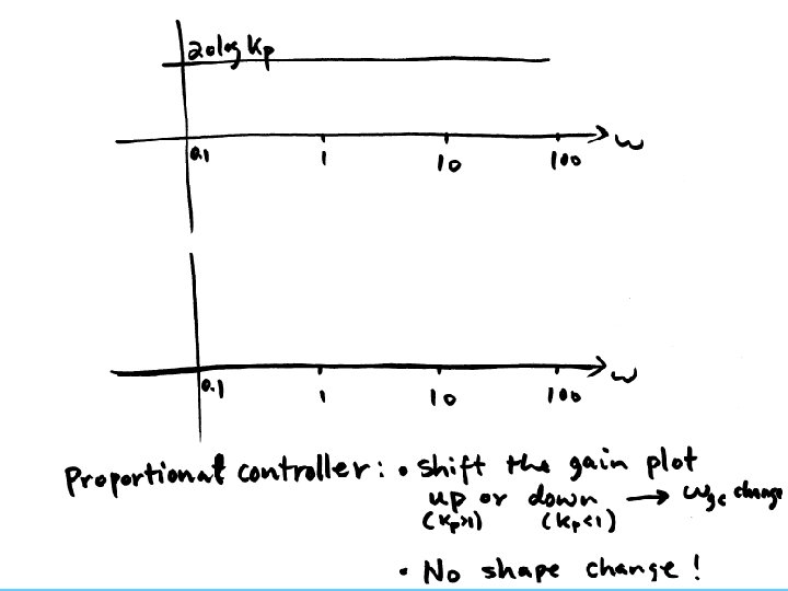
Proportional controller design • Obtain open loop Bode plot • Convert design specs into Bode plot req. • Select KP based on requirements: – For improving ess: KP = Kp, v, a, des / Kp, v, a, act – For fixing Mp: select wgcd to be the freq at which PM is sufficient, and KP = 1/|G(jwgcd)| – For fixing speed: from td, tr, tp, or ts requirement, find out wn, let wgcd = wn and choose KP as above
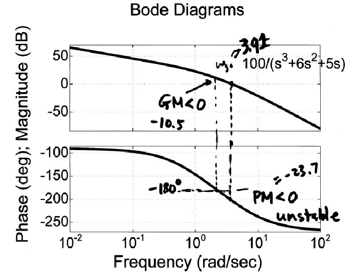
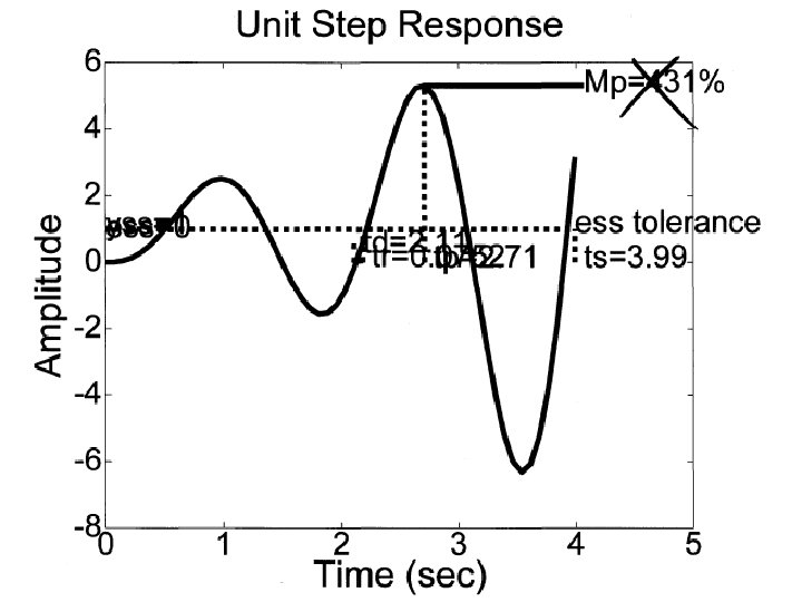
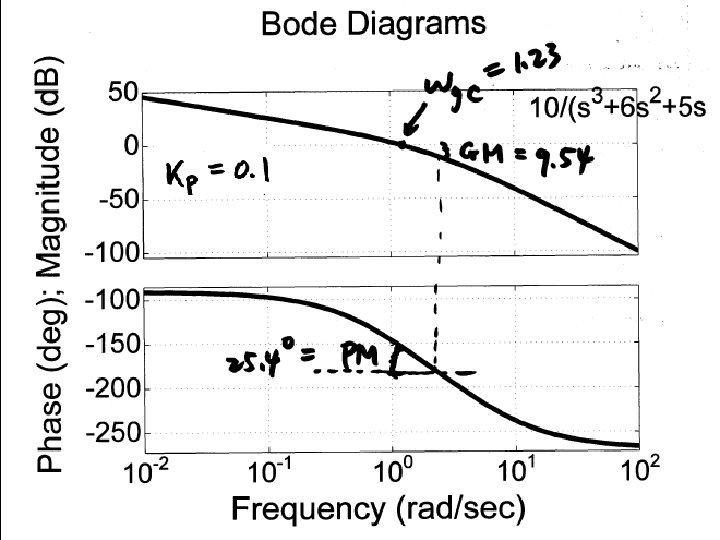
clear all; n=[0 0 40]; d=[1 2 0]; figure(1); clf; margin(n, d); %proportional control design: figure(1); hold on; grid; V=axis; Mp = 10; %overshoot in percentage PMd = 70 -Mp + 3; semilogx(V(1: 2), [PMd-180], ': r'); %get desired w_gc x=ginput(1); w_gcd = x(1); KP = 1/abs(evalfr(tf(n, d), j*w_gcd)); figure(2); margin(KP*n, d); figure(3); mystep(KP*n, d+KP*n);
Lead Controller Design
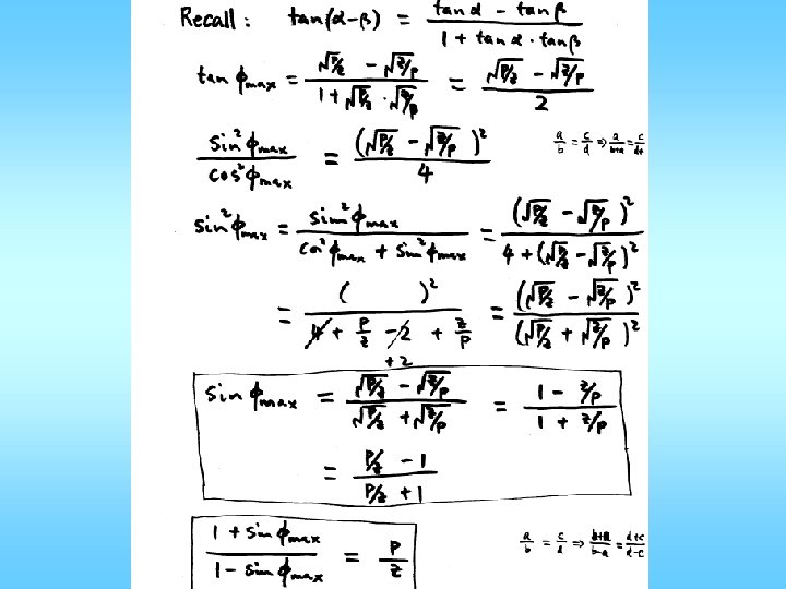
plead zlead 20 log(Kzlead/plead) Goal: select z and p so that max phase lead is at desired wgc and max phase lead = PM defficiency!
Lead Design • • • From specs => PMd and wgcd From plant, draw Bode plot Find PMhave = 180 + angle(G(jwgcd) DPM = PMd - PMhave + a few degrees Choose a=plead/zlead so that fmax = DPM and it happens at wgcd
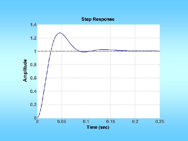
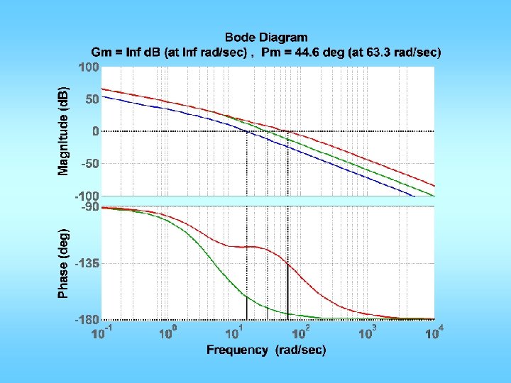
Lead design example • Plant transfer function is given by: • n=[50000]; d=[1 60 500 0]; • Desired design specifications are: – Step response overshoot <= 16% – Closed-loop system BW>=20;
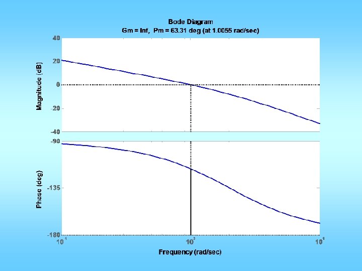
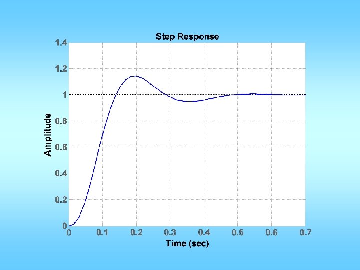
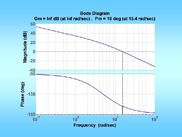
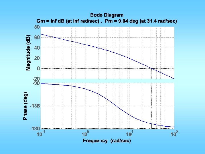
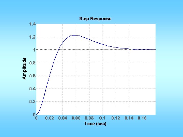
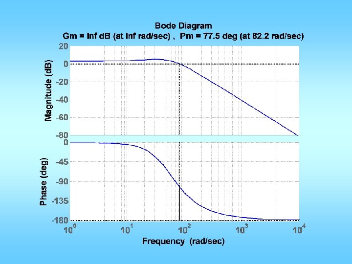
n=[50000]; d=[1 60 500 0]; G=tf(n, d); figure(1); margin(G); Mp_d = 16/100; zeta_d =0. 5; % or calculate from Mp_d PMd = 100*zeta_d + 3; BW_d=20; w_gcd = BW_d*0. 7; Gwgc=evalfr(G, j*w_gcd); PM = pi+angle(Gwgc); phimax= PMd*pi/180 -PM; alpha=(1+sin(phimax))/(1 -sin(phimax)); zlead= w_gcd/sqrt(alpha); plead=w_gcd*sqrt(alpha); K=sqrt(alpha)/abs(Gwgc); ngc = conv(n, K*[1 zlead]); dgc = conv(d, [1 plead]); figure(1); hold on; margin(ngc, dgc); hold off; [ncl, dcl]=feedback(ngc, dgc, 1, 1); figure(2); step(ncl, dcl);
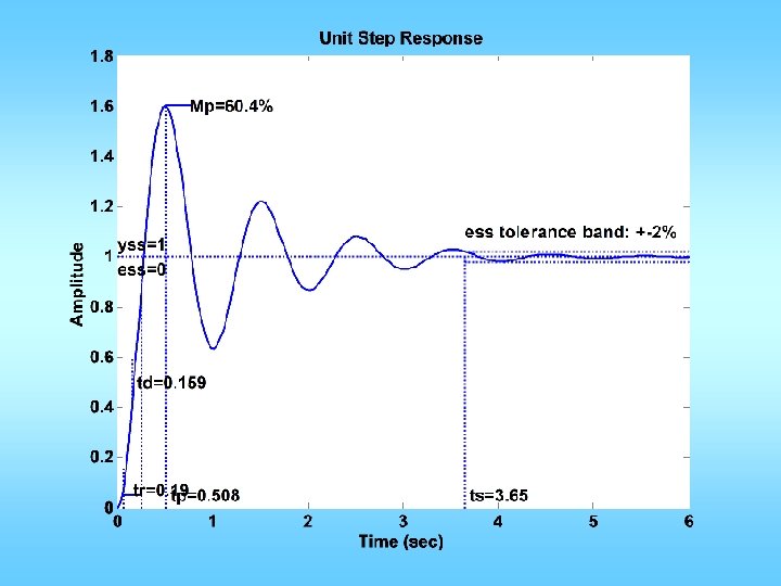
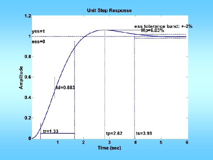
Before design After design
Closed-loop Bode plot by: margin(ncl*1. 414, dcl); Magnitude plot shifted up 3 So, gc is BW
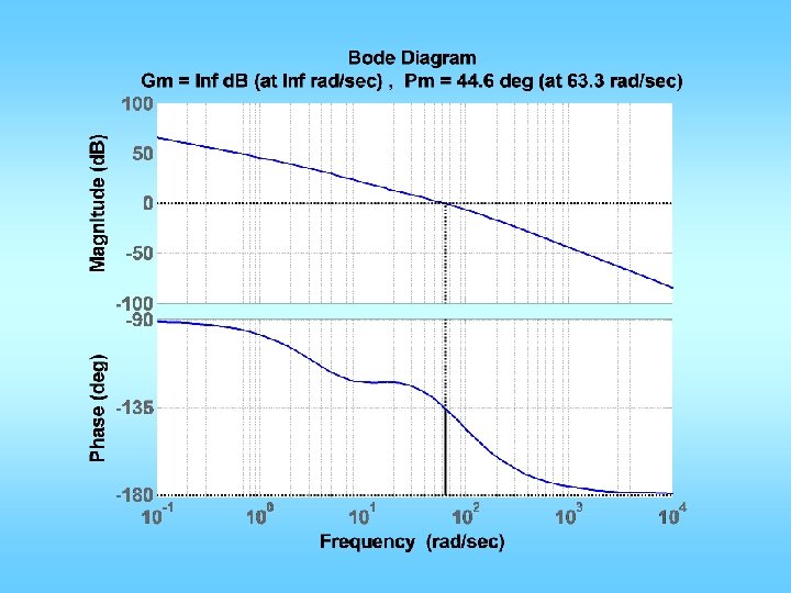
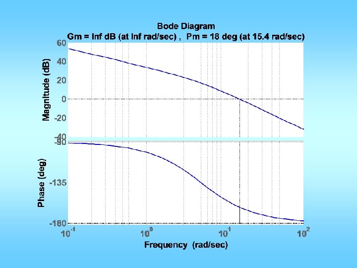
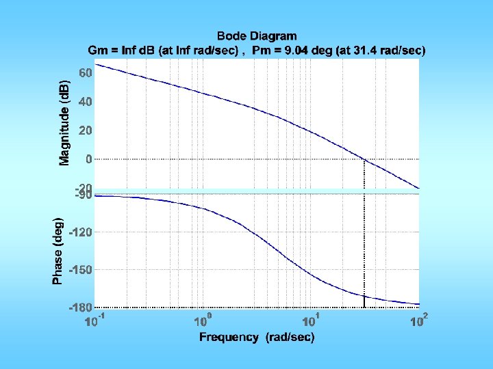
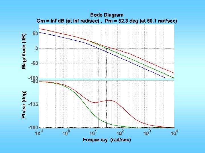
n=[50]; d=[1/5 1 0]; figure(1); clf; margin(n, d); grid; hold on; Mp = 20/100; zeta = sqrt((log(Mp))^2/(pi^2+(log(Mp))^2)); PMd = zeta * 100 + 10; ess 2 ramp= 1/200; Kvd=1/ess 2 ramp; Kva = n(end)/d(end-1); Kzp = Kvd/Kva; figure(2); margin(Kzp*n, d); grid; [GM, PM, wpc, wgc]=margin(Kzp*n, d); w_gcd=wgc; phimax = (PMd-PM)*pi/180; alpha=(1+sin(phimax))/(1 -sin(phimax)); z=w_gcd/sqrt(alpha); p=w_gcd*sqrt(alpha); ngc = conv(n, alpha*Kzp*[1 z]); dgc = conv(d, [1 p]); figure(3); margin(tf(ngc, dgc)); grid; [ncl, dcl]=feedback(ngc, dgc, 1, 1); figure(4); step(ncl, dcl); grid; figure(5); margin(ncl*1. 414, dcl); grid;
n=[50]; d=[1/5 1 0]; figure(1); clf; margin(n, d); grid; hold on; Mp = 20/100; zeta = sqrt((log(Mp))^2/(pi^2+(log(Mp))^2)); PMd = zeta * 100 + 10; ess 2 ramp= 1/200; Kvd=1/ess 2 ramp; Kva = n(end)/d(end-1); Kzp = Kvd/Kva; figure(2); margin(Kzp*n, d); grid; [GM, PM, wpc, wgc]=margin(Kzp*n, d); w_gcd=wgc; phimax = (PMd-PM)*pi/180; alpha=(1+sin(phimax))/(1 -sin(phimax)); z=w_gcd/alpha^. 25; %sqrt(alpha); p=w_gcd*alpha^. 75; %sqrt(alpha); ngc = conv(n, alpha*Kzp*[1 z]); dgc = conv(d, [1 p]); figure(3); margin(tf(ngc, dgc)); grid; [ncl, dcl]=feedback(ngc, dgc, 1, 1); figure(4); step(ncl, dcl); grid; figure(5); margin(ncl*1. 414, dcl); grid;