Introduction to Image Compression Run Length Encoding Data

Introduction to Image Compression

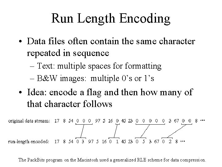
Run Length Encoding • Data files often contain the same character repeated in sequence – Text: multiple spaces formatting – B&W images: multiple 0’s or 1’s • Idea: encode a flag and then how many of that character follows The Pack. Bits program on the Macintosh used a generalized RLE scheme for data compression.

Arithmetic Encoding • Turn an entire datastream into a single number – The more data we have, the greater precision we will need in representing the number. – There are two fundamentals in arithmetic coding • The probability of a symbol • A symbol’s encoding interval range

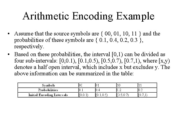
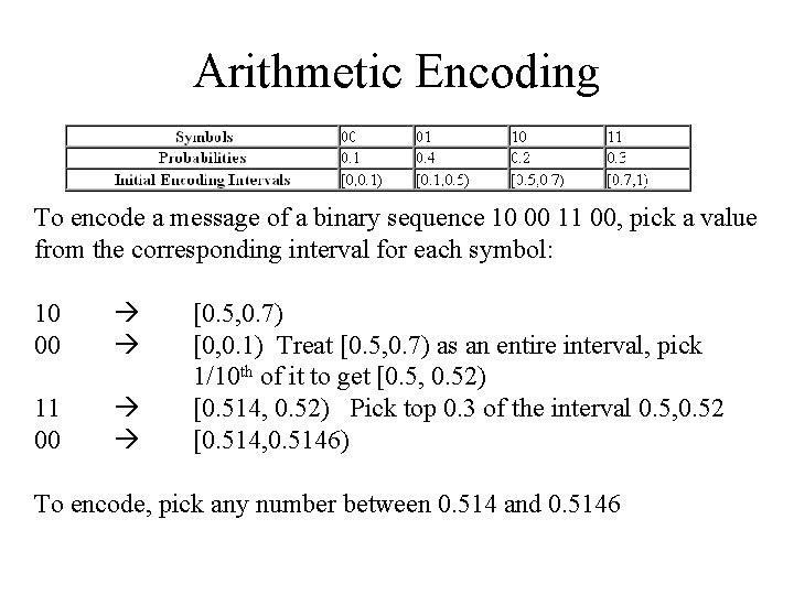
Arithmetic Encoding Example • Assume that the source symbols are { 00, 01, 10, 11 } and the probabilities of these symbols are { 0. 1, 0. 4, 0. 2, 0. 3 }, respectively. • Based on these probabilities, the interval [0, 1) can be divided as four sub-intervals: [0, 0. 1), [0. 1, 0. 5), [0. 5, 0. 7), [0. 7, 1), where [x, y) denotes a half open interval, which includes x but excludes y. The above information can be summarized in the table:

Arithmetic Encoding To encode a message of a binary sequence 10 00 11 00, pick a value from the corresponding interval for each symbol: 10 00 11 00 [0. 5, 0. 7) [0, 0. 1) Treat [0. 5, 0. 7) as an entire interval, pick 1/10 th of it to get [0. 5, 0. 52) [0. 514, 0. 52) Pick top 0. 3 of the interval 0. 5, 0. 52 [0. 514, 0. 5146) To encode, pick any number between 0. 514 and 0. 5146

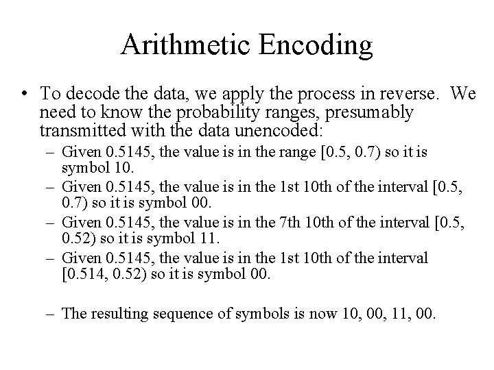
Arithmetic Encoding • To decode the data, we apply the process in reverse. We need to know the probability ranges, presumably transmitted with the data unencoded: – Given 0. 5145, the value is in the range [0. 5, 0. 7) so it is symbol 10. – Given 0. 5145, the value is in the 1 st 10 th of the interval [0. 5, 0. 7) so it is symbol 00. – Given 0. 5145, the value is in the 7 th 10 th of the interval [0. 5, 0. 52) so it is symbol 11. – Given 0. 5145, the value is in the 1 st 10 th of the interval [0. 514, 0. 52) so it is symbol 00. – The resulting sequence of symbols is now 10, 00, 11, 00.

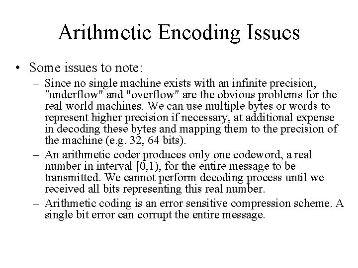
Arithmetic Encoding Issues • Some issues to note: – Since no single machine exists with an infinite precision, "underflow" and "overflow" are the obvious problems for the real world machines. We can use multiple bytes or words to represent higher precision if necessary, at additional expense in decoding these bytes and mapping them to the precision of the machine (e. g. 32, 64 bits). – An arithmetic coder produces only one codeword, a real number in interval [0, 1), for the entire message to be transmitted. We cannot perform decoding process until we received all bits representing this real number. – Arithmetic coding is an error sensitive compression scheme. A single bit error can corrupt the entire message.

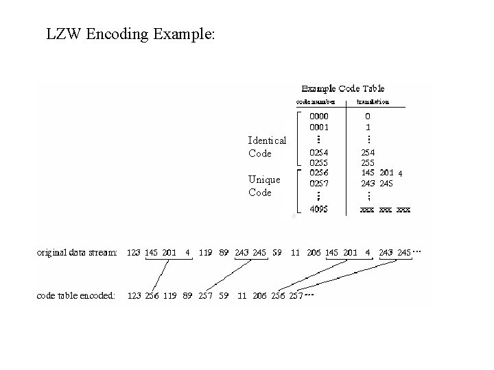
LZW Encoding • Popular form of compression that is used as the basis for many commercial and non-commercial compression programs – gzip, pkzip, GIF, compressed postscript, “disk doublers” • Developers – A. Lempel and J. Ziv, with later modifications by Terry A. Welch • LZW is similar to Huffman encoding, except it uses a code table for sequences of characters

LZW Encoding Example: Identical Code Unique Code

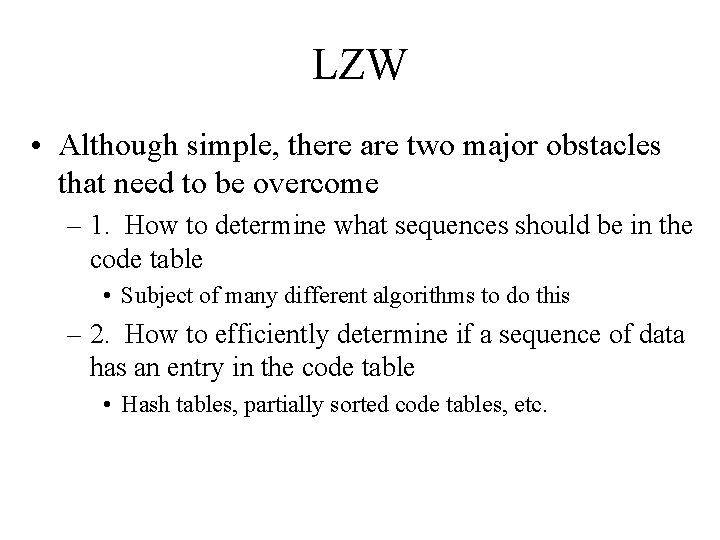
LZW • Although simple, there are two major obstacles that need to be overcome – 1. How to determine what sequences should be in the code table • Subject of many different algorithms to do this – 2. How to efficiently determine if a sequence of data has an entry in the code table • Hash tables, partially sorted code tables, etc.

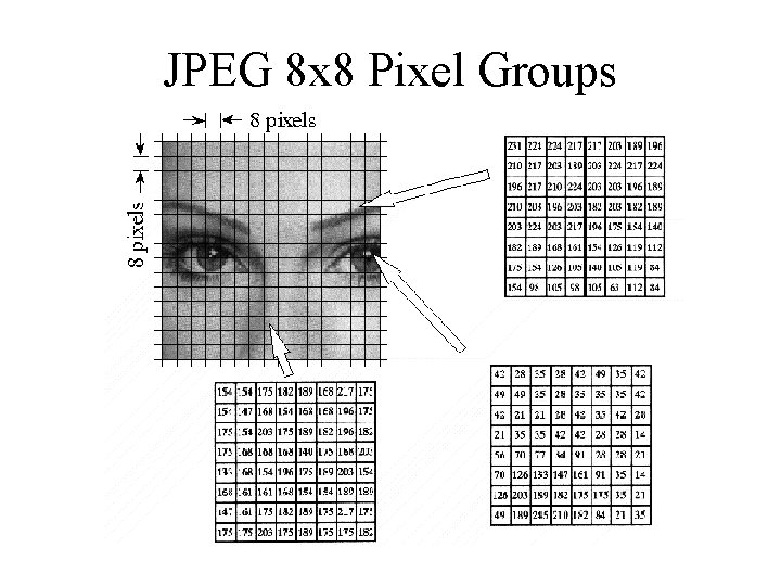
JPEG • Lossy compression – A family of techniques called transform compression has proven the most valuable – Named after its originating group, the Joint Photographers Experts Group • JPEG compression starts by breaking the image into 8 x 8 pixel groups. – The full JPEG algorithm can accept a wide range of bits per pixel, including the use of color information. In our example, each pixel is a single byte, a grayscale value between 0 and 255. – Each 8 x 8 pixel groups are treated independently during compression. – Why use 8 x 8 pixel groups instead of, for instance, 16 x 16? • Maximum size that integrated circuit technology could handle at the time the standard was developed • Seems to work fairly well

JPEG 8 x 8 Pixel Groups

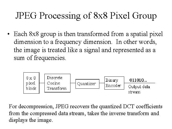
JPEG Processing of 8 x 8 Pixel Group • Each 8 x 8 group is then transformed from a spatial pixel dimension to a frequency dimension. In other words, the image is treated like a signal and represented as a sum of frequencies. For decompression, JPEG recovers the quantized DCT coefficients from the compressed data stream, takes the inverse transform and displays the image.

Discrete Cosine Transform (DCT) • Key to the JPEG compression process • The DCT is in a class of mathematical operations that includes the well known Fast Fourier Transform (FFT) and many others (e. g. wavelets) • Basic purpose – Take a signal and transform it from a spatial representation of pixels into frequencies of waves, or “spectral” information, so that it can be manipulated for compression. – Compressed by discarding or approximating information that is not perceivable by the human eye – Translate from the spatial to frequency domain • The signal for a graphical image can be thought of as a three-dimensional signal. – X/Y axis of the image’s signal are the two dimensions of the screen – Z axis is the amplitude of the signal, or the pixel’s value at (X, Y) • Start with a 1 dimensional signal

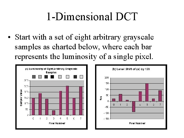
1 -Dimensional DCT • Start with a set of eight arbitrary grayscale samples as charted below, where each bar represents the luminosity of a single pixel.

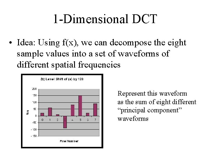
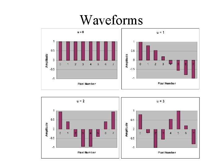
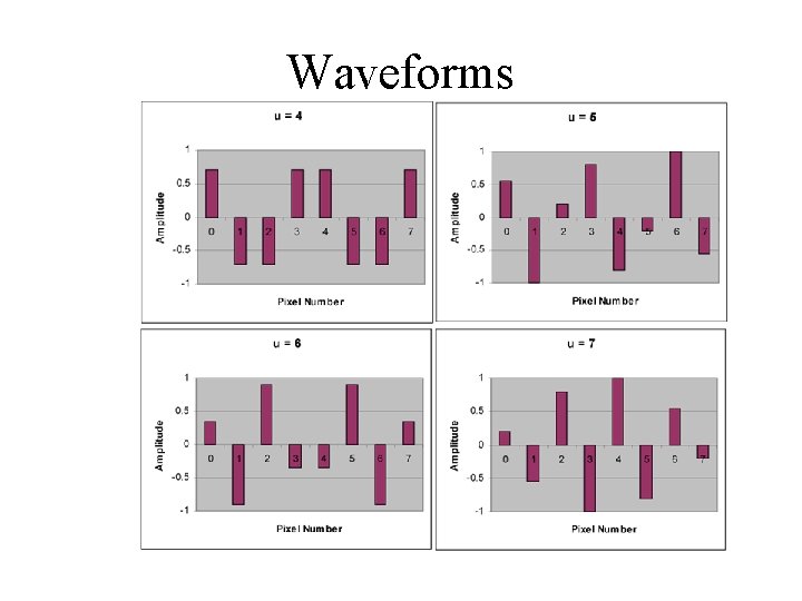
1 -Dimensional DCT • Idea: Using f(x), we can decompose the eight sample values into a set of waveforms of different spatial frequencies Represent this waveform as the sum of eight different “principal component” waveforms

Waveforms

Waveforms

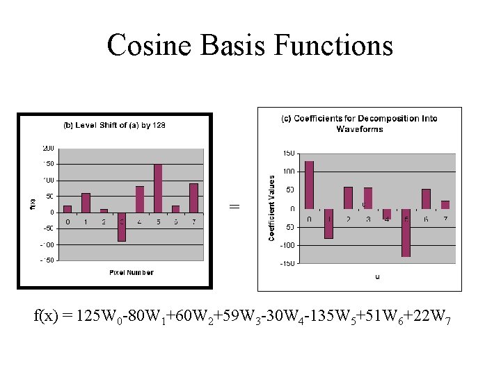
Cosine Basis Functions • Waveforms show an alternating behavior at progressively higher frequencies • These waveforms, which are called cosine basis functions, are independent – There is no way that one of the eight waveforms can be represented by any combination of the other waveforms • However, the complete set of eight waveforms, when scaled by coefficients and added together, can be used to represent any eight sample values

Cosine Basis Functions = f(x) = 125 W 0 -80 W 1+60 W 2+59 W 3 -30 W 4 -135 W 5+51 W 6+22 W 7

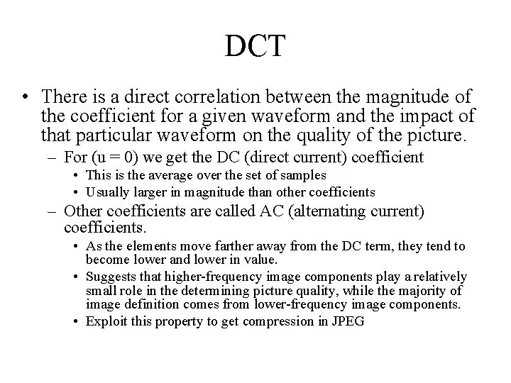
DCT • There is a direct correlation between the magnitude of the coefficient for a given waveform and the impact of that particular waveform on the quality of the picture. – For (u = 0) we get the DC (direct current) coefficient • This is the average over the set of samples • Usually larger in magnitude than other coefficients – Other coefficients are called AC (alternating current) coefficients. • As the elements move farther away from the DC term, they tend to become lower and lower in value. • Suggests that higher-frequency image components play a relatively small role in the determining picture quality, while the majority of image definition comes from lower-frequency image components. • Exploit this property to get compression in JPEG

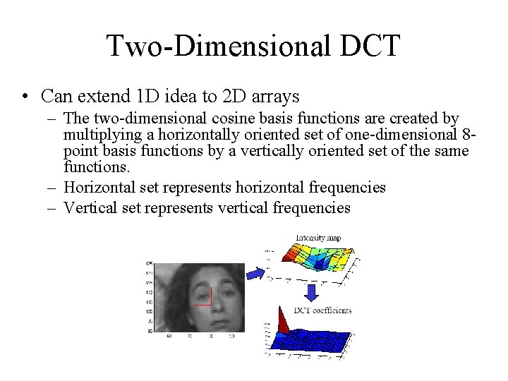
Two-Dimensional DCT • Can extend 1 D idea to 2 D arrays – The two-dimensional cosine basis functions are created by multiplying a horizontally oriented set of one-dimensional 8 point basis functions by a vertically oriented set of the same functions. – Horizontal set represents horizontal frequencies – Vertical set represents vertical frequencies

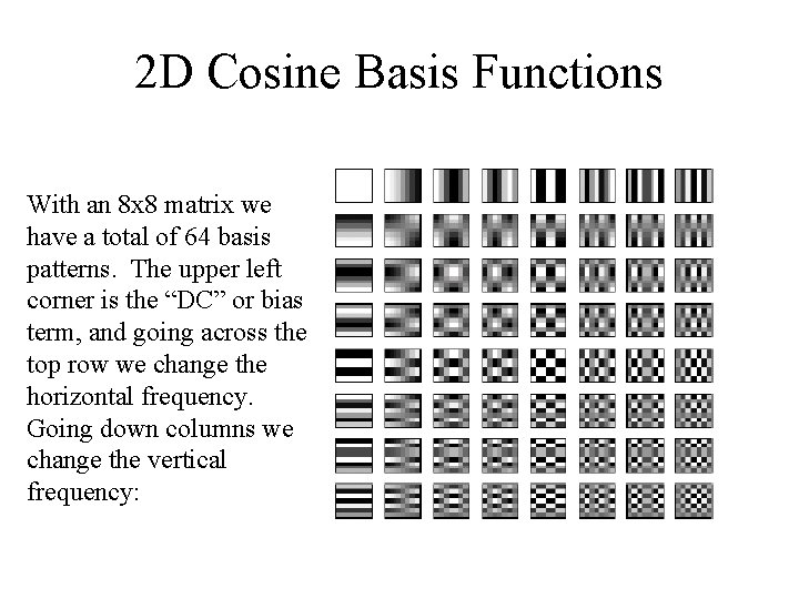
2 D Cosine Basis Functions With an 8 x 8 matrix we have a total of 64 basis patterns. The upper left corner is the “DC” or bias term, and going across the top row we change the horizontal frequency. Going down columns we change the vertical frequency:

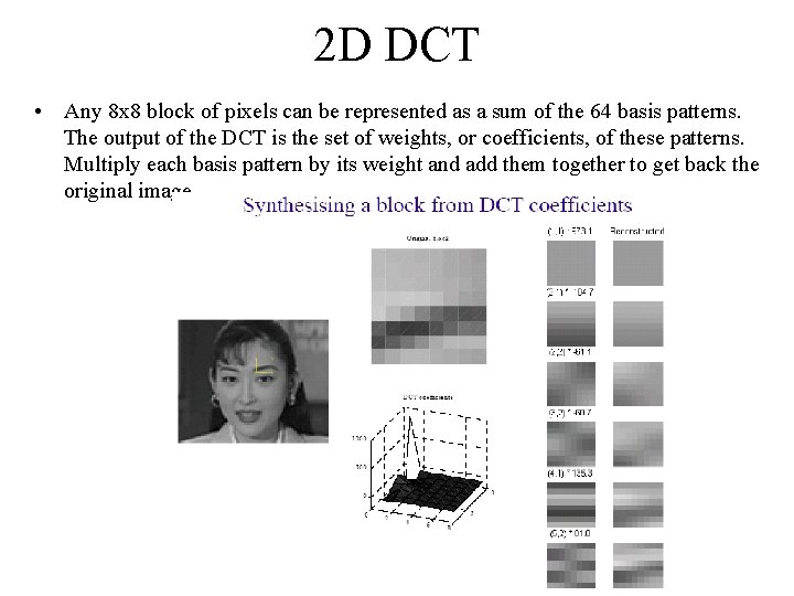
2 D DCT • Any 8 x 8 block of pixels can be represented as a sum of the 64 basis patterns. The output of the DCT is the set of weights, or coefficients, of these patterns. Multiply each basis pattern by its weight and add them together to get back the original image.

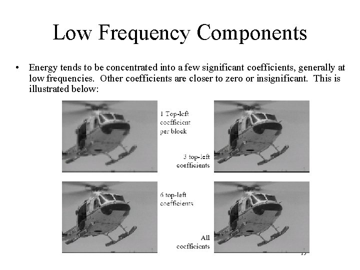
Low Frequency Components • Energy tends to be concentrated into a few significant coefficients, generally at low frequencies. Other coefficients are closer to zero or insignificant. This is illustrated below:

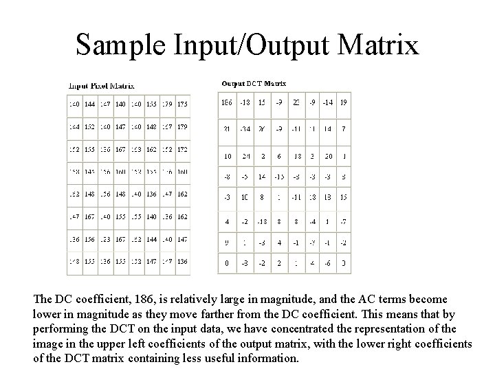
Sample Input/Output Matrix The DC coefficient, 186, is relatively large in magnitude, and the AC terms become lower in magnitude as they move farther from the DC coefficient. This means that by performing the DCT on the input data, we have concentrated the representation of the image in the upper left coefficients of the output matrix, with the lower right coefficients of the DCT matrix containing less useful information.

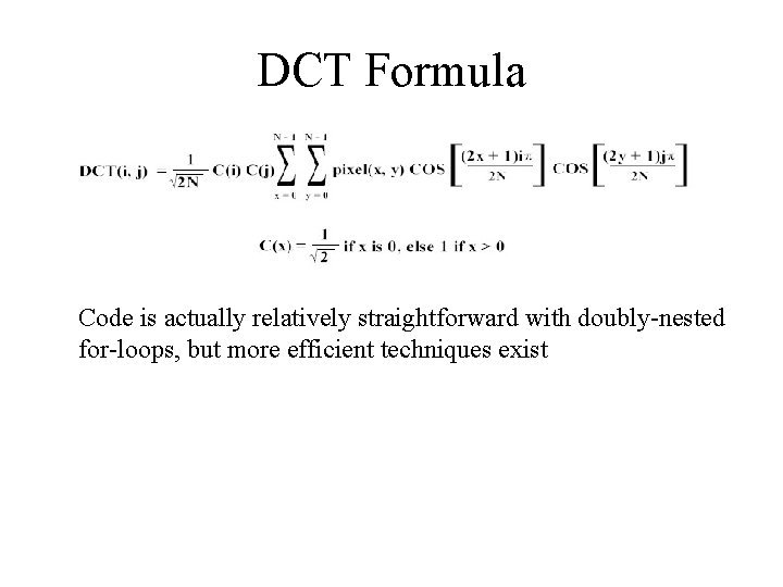
DCT Formula Code is actually relatively straightforward with doubly-nested for-loops, but more efficient techniques exist

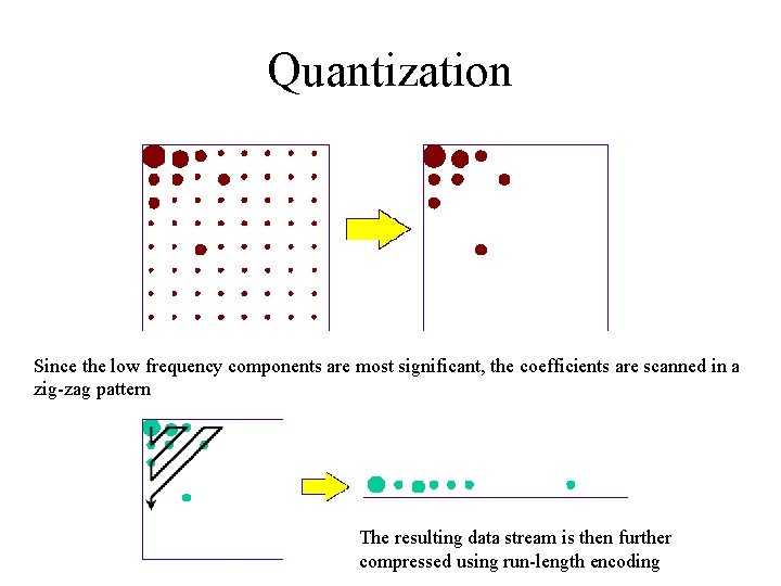
Coefficient Quantization • Quantization is the process of reducing the number of bits needed to store an integer value by reducing the precision of the integer. – Given a matrix of DCT coefficients, we generally reduce the precision of the coefficients more and more as we move away from the DC coefficient. • The algorithm essentially divides each DCT coefficient by an integer and discards the remainder. The result is a loss of precision, but fewer bits that we need to store. Typically, only a few non-zero coefficients are left.

Quantization Since the low frequency components are most significant, the coefficients are scanned in a zig-zag pattern The resulting data stream is then further compressed using run-length encoding

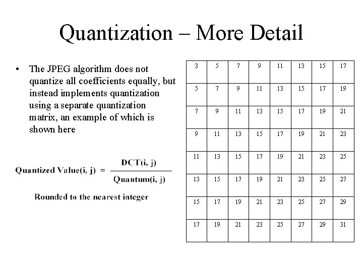
Quantization – More Detail • The JPEG algorithm does not quantize all coefficients equally, but instead implements quantization using a separate quantization matrix, an example of which is shown here 3 5 7 9 11 13 15 17 19 21 23 11 13 15 17 19 21 23 25 27 29 31

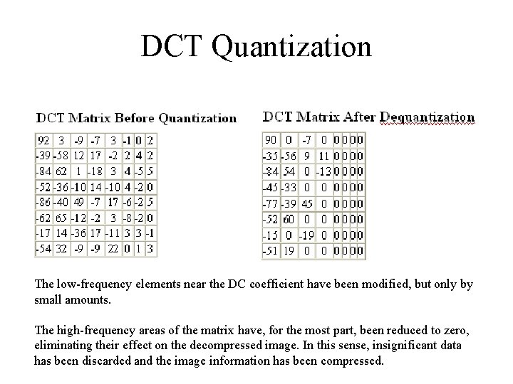
DCT Quantization The low-frequency elements near the DC coefficient have been modified, but only by small amounts. The high-frequency areas of the matrix have, for the most part, been reduced to zero, eliminating their effect on the decompressed image. In this sense, insignificant data has been discarded and the image information has been compressed.

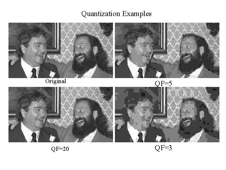
How to pick the quantization values? • An enormous number of schemes could be used to define these values, and the two most common experimental approaches for testing the effectiveness of such schemes are as follows: – Measure the mathematical error found between an input image and its output image after it has been decompressed, trying to determine an acceptable level of error. – Simply "eyeball it". Although judging the effect of decompression on the human eye is purely subjective, it may, in some cases, be more credible than mathematical differences in error levels. • Although JPEG allows for the use of any quantization matrix, ISO has done extensive testing and developed a standard set of quantization values that cause impressive degrees of compression.

Quantization Examples Original QF=20 QF=5 QF=3