Macroeconomic Topics in Development Transition EC 938 Sharun

Macroeconomic Topics in Development & Transition EC 938 Sharun W. Mukand 1

Development Policy and Macroeconomics 2 l Economic Growth l Globalization, Trade and Inequality l Political and Economic Crises: Currency Crises l Governance and Institutions l Political Economy of Policymaking l Foreign Aid, Corruption l Miscellaneous Topics

3 l Background: Some stylized facts about developing countries (macroeconomy) l Economic Growth…. Theory + evidence -- proximate versus ultimate causes -- growth and policymaking.

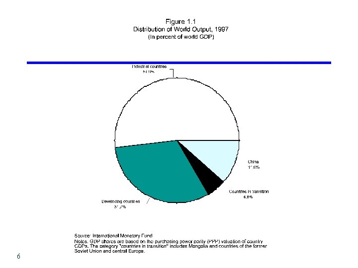
Some stylized facts (Macro)…. l l l 4 In 1997 developing countries accounted for 32% of world output. 132 of the 183 countries are developing countries. Although most of production takes place in the industrial countries, country-specific macroeconomic policy formulation is carried out in a developing-country context. Developing countries behave similarly to industrial countries, but operate in a different environment. Emphasis on politics, reputation, credibility, inequality, exchange rate management, crises….

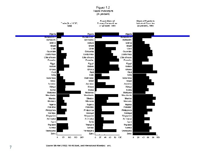
Stylized facts (contd…) 1. Developing economies tend to be more open to trade in l l l 5 goods and services than are the major industrial countries. Openness: trade share (sum of the shares of exports and imports) in GDP. First panel of Figure 1. 2: developing nations tend to be more open than the major industrial countries. Mean value of the trade share is 45%, compared with about 25% in the G-7 countries.

6

7

2. Developing countries typically have little control over the prices of the goods they export and import. Exogeneity of the terms of trade is suggested both è by their small share in the world economy; è by the composition of their exports. In 1990 developing nations accounted for about one quarter of world exports and imports. In 1991 over half of the exports of low- and middle-income countries consisted of primary commodities. Second panel of Figure 1. 2: share of primary commodities in the exports of a selected group of developing countries. Third panel: two-thirds of the exports of the countries went to industrial countries. l l l 8

9

3. Extent of external trade in assets has been more limited in developing countries, though this situation has recently begun to change. l l l 10 Developing countries have undergone an increase in their degree of integration with the world capital market. Integration occurred in the context of immature domestic financial systems, limited policy flexibility, and fragile credibility. This situation has caused to the capital inflow problem in some countries.

4. Majority of developing countries have neither adopted fully flexible exchange rates nor joined monetary unions. l l l 11 In developing countries officially determined rates predominate. Exchange regimes in developing countries have evolved toward greater flexibility since the collapse of the Bretton Woods system in 1973. This has meant that more frequent adjustments of an officially determined parity rather than the adoption of market-determined exchange rates.

Domestic Financial Markets 5. Financial markets in developing nations have been characterized by the prevalence of rudimentary financial institutions and by “financial repression. l l l 12 Only some of the developing countries have developed large equity markets. Financial markets are dominated by commercial banks. Equity markets tend to be dominated by a few firms and exhibit very low turnover.

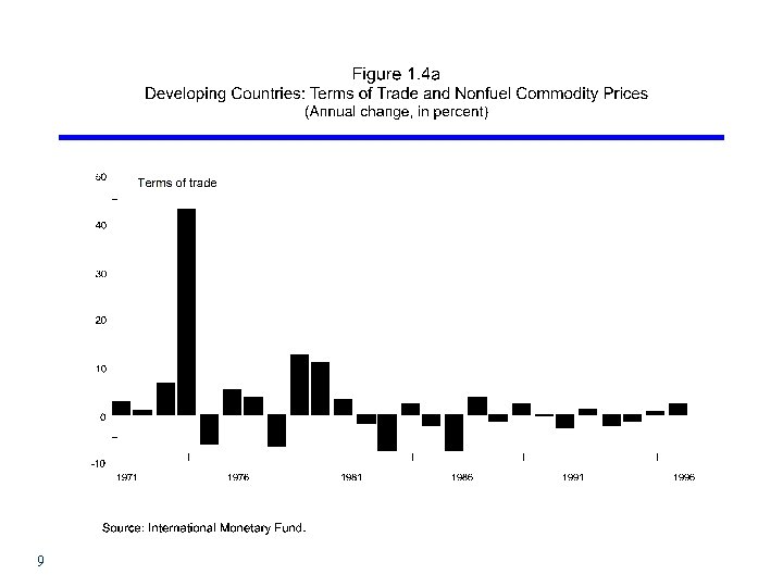
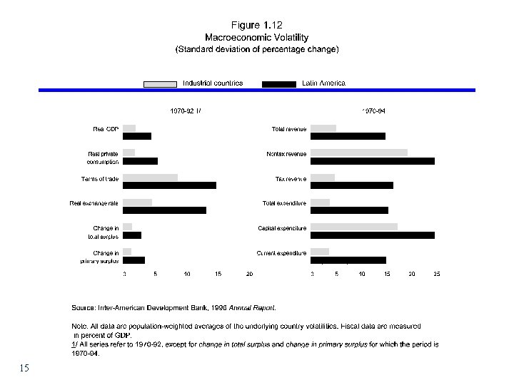
Macroeconomic Volatility 6. Macroeconomic environment in developing countries is much more volatile. Roots of macroeconomic instability are both external and internal: è Volatility in the terms of trade and international financial conditions. è Inflexibility of domestic macroeconomic instruments and political instability. Figure 1. 12: l Latin America case. l All components of the governments budget is less stable. l 13

Politics Matters! l 14 Policymaking in developing/transition countries is vulnerable to political factors to a far greater extent than in developed countries.

15

l l 16 Gavin and Perotti (1997): volatility in some Latin American countries have been compounded by a procyclical fiscal policy response: è increase in government expenditure and fiscal deficits during periods of expansion; è fall during recessions. Overall, boom and bust phenomena tend to be much more common and more costly in developing countries. Why?

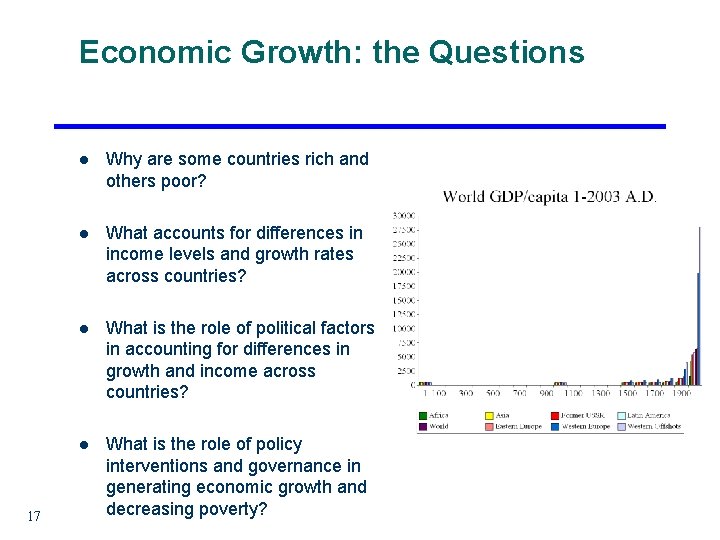
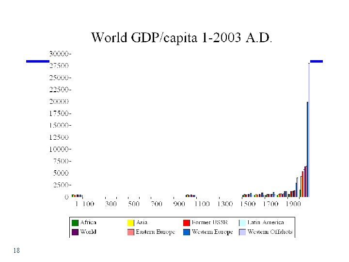
Economic Growth: the Questions 17 l Why are some countries rich and others poor? l What accounts for differences in income levels and growth rates across countries? l What is the role of political factors in accounting for differences in growth and income across countries? l What is the role of policy interventions and governance in generating economic growth and decreasing poverty?

18

Economic Growth ü Present a policy-oriented overview of theory and empirical evidence of economic growth ü ü 19 Trace linkages between economic growth and its main determinants: (i) proximate: saving, investment, and economic efficiency (ii) ultimate(? ): Institutions, culture, geography….

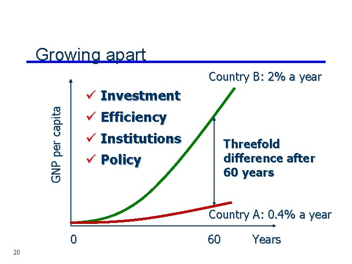
Growing apart Country B: 2% a year GNP per capita ü Investment ü Efficiency ü Institutions ü Policy Threefold difference after 60 years Country A: 0. 4% a year 0 20 60 Years

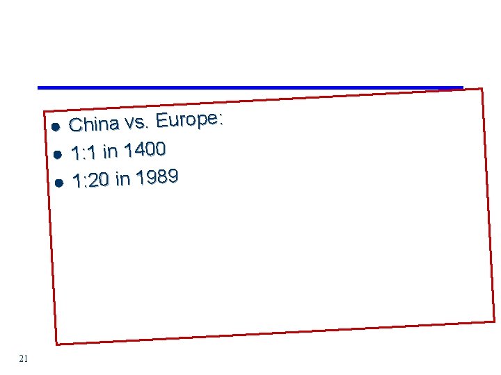
China vs. Europe: l 1: 1 in 1400 l 1: 20 in 1989 l 21

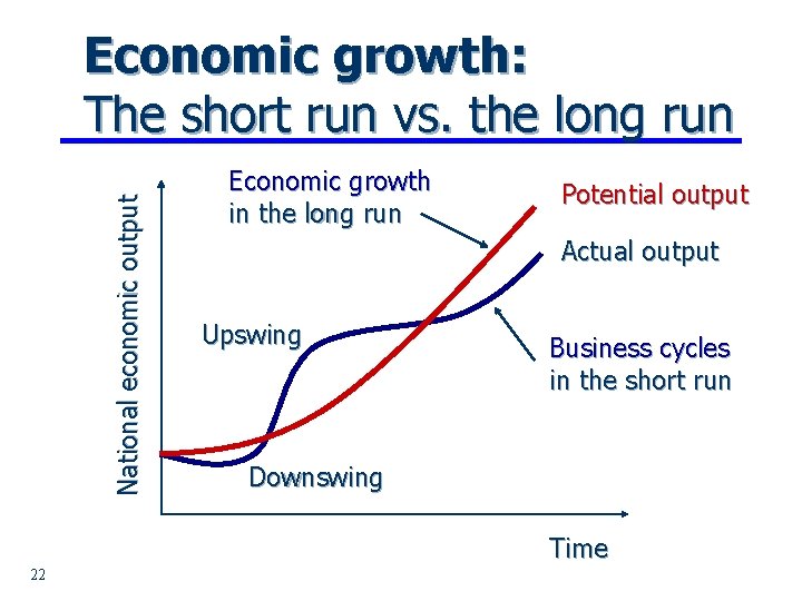
National economic output Economic growth: The short run vs. the long run Economic growth in the long run Potential output Actual output Upswing Business cycles in the short run Downswing Time 22

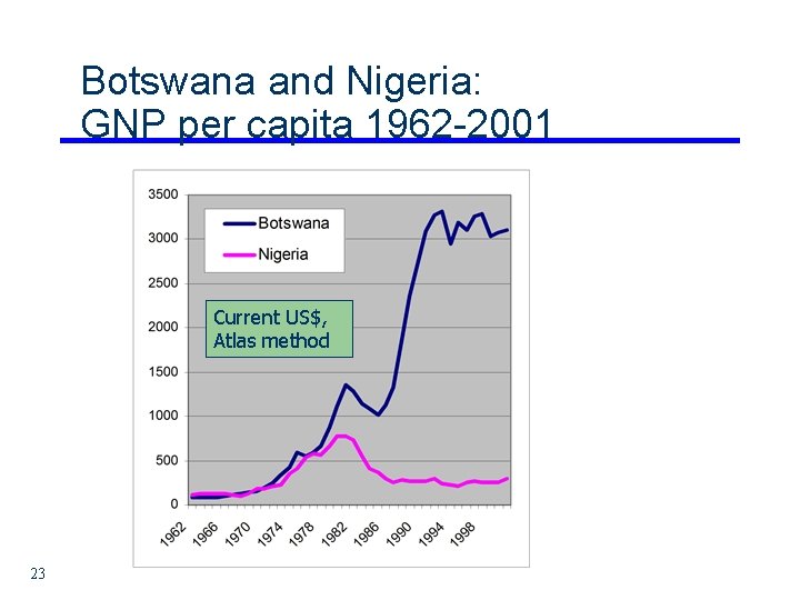
Botswana and Nigeria: GNP per capita 1962 -2001 Current US$, Atlas method 23

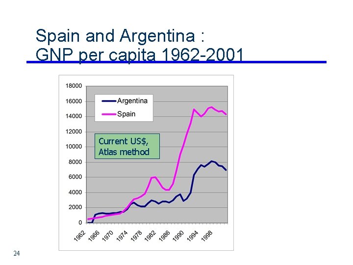
Spain and Argentina : GNP per capita 1962 -2001 Current US$, Atlas method 24

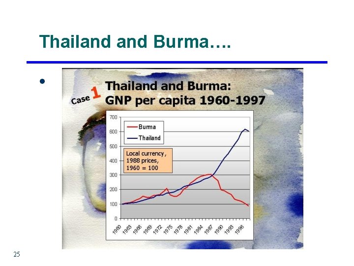
Thailand Burma…. l 25

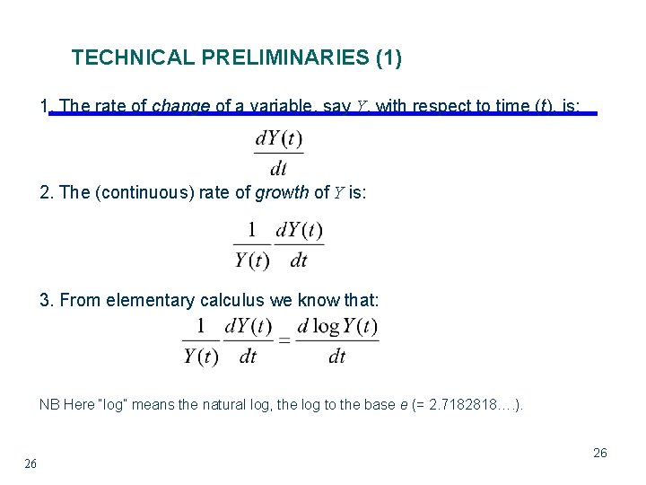
TECHNICAL PRELIMINARIES (1) 1. The rate of change of a variable, say Y, with respect to time (t), is: 2. The (continuous) rate of growth of Y is: 3. From elementary calculus we know that: NB Here “log” means the natural log, the log to the base e (= 2. 7182818…. ). 26 26

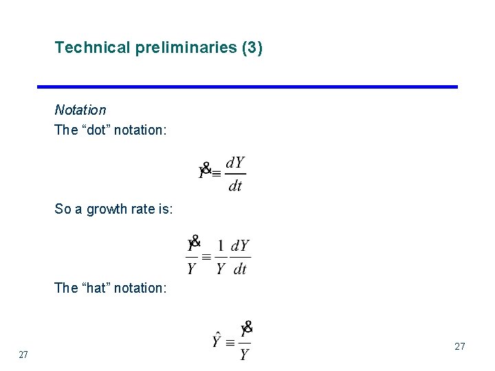
Technical preliminaries (3) Notation The “dot” notation: So a growth rate is: The “hat” notation: 27 27

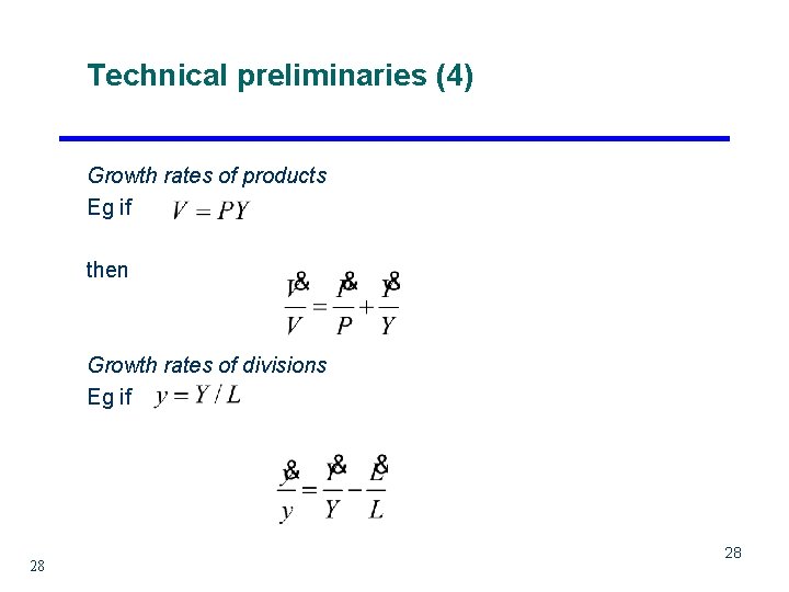
Technical preliminaries (4) Growth rates of products Eg if then Growth rates of divisions Eg if 28 28

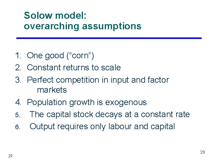
Solow model: overarching assumptions 1. One good (“corn”) 2. Constant returns to scale 3. Perfect competition in input and factor markets 4. Population growth is exogenous 5. The capital stock decays at a constant rate 6. Output requires only labour and capital 29 29

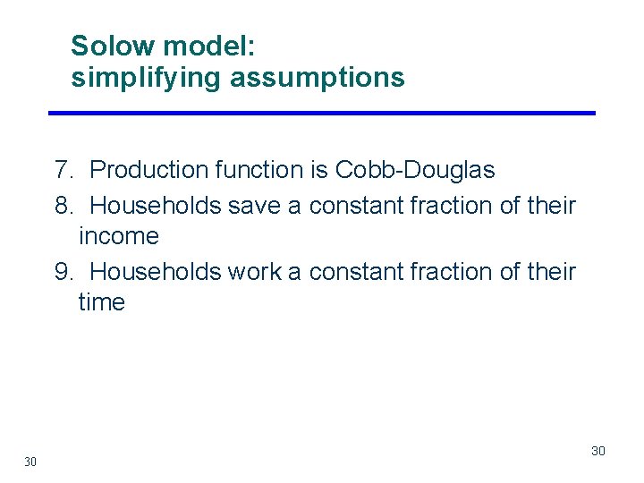
Solow model: simplifying assumptions 7. Production function is Cobb-Douglas 8. Households save a constant fraction of their income 9. Households work a constant fraction of their time 30 30

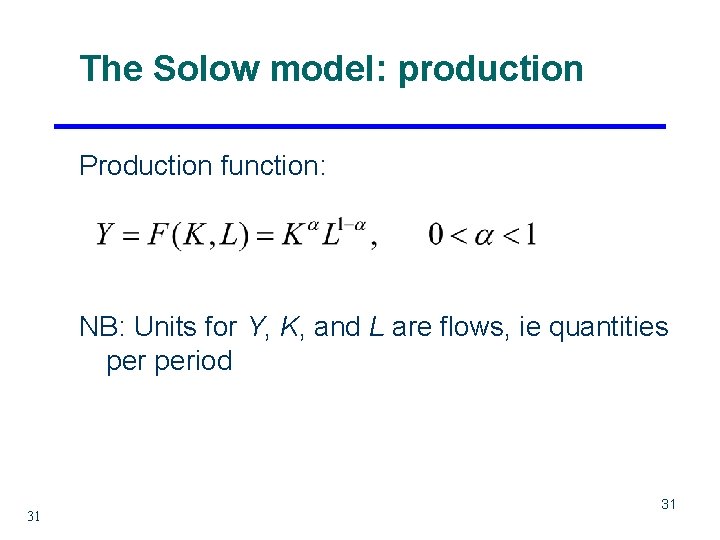
The Solow model: production Production function: NB: Units for Y, K, and L are flows, ie quantities period 31 31

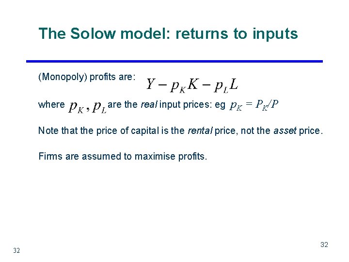
The Solow model: returns to inputs (Monopoly) profits are: where are the real input prices: eg p. K = PK/P Note that the price of capital is the rental price, not the asset price. Firms are assumed to maximise profits. 32 32

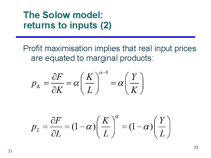
The Solow model: returns to inputs (2) Profit maximisation implies that real input prices are equated to marginal products: 33 33

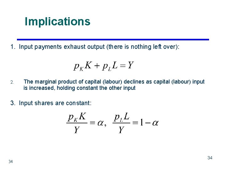
Implications 1. Input payments exhaust output (there is nothing left over): 2. The marginal product of capital (labour) declines as capital (labour) input is increased, holding constant the other input 3. Input shares are constant: 34 34

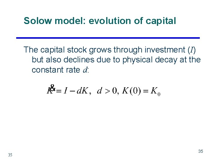
Solow model: evolution of capital The capital stock grows through investment (I) but also declines due to physical decay at the constant rate d: 35 35

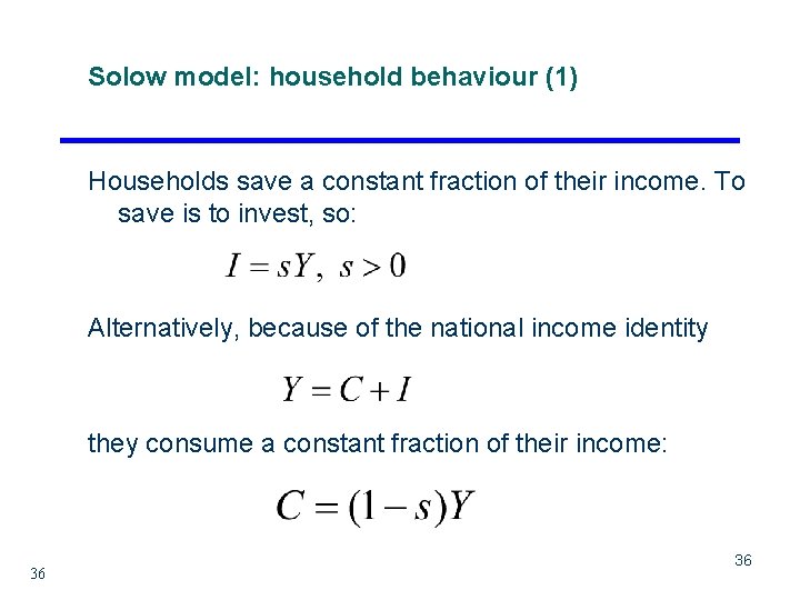
Solow model: household behaviour (1) Households save a constant fraction of their income. To save is to invest, so: Alternatively, because of the national income identity they consume a constant fraction of their income: 36 36

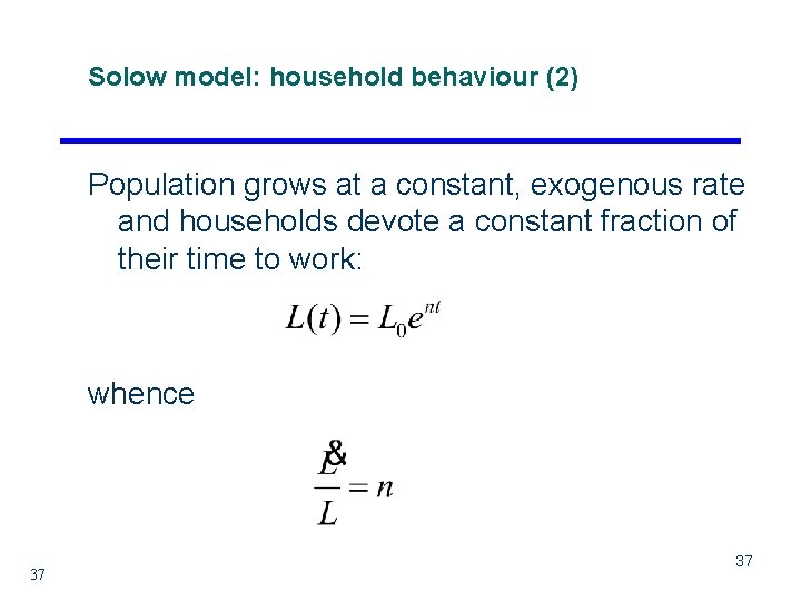
Solow model: household behaviour (2) Population grows at a constant, exogenous rate and households devote a constant fraction of their time to work: whence 37 37

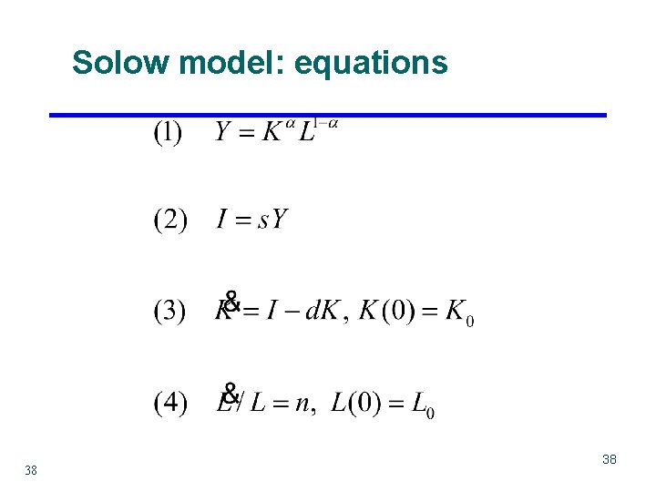
Solow model: equations 38 38

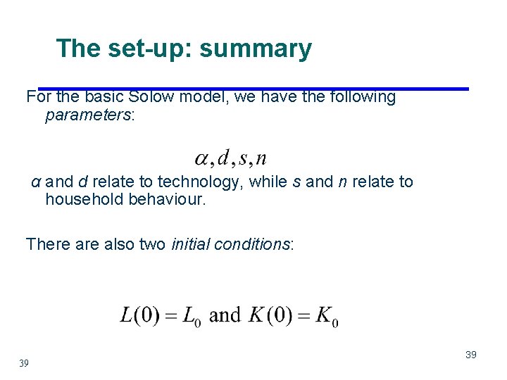
The set-up: summary For the basic Solow model, we have the following parameters: α and d relate to technology, while s and n relate to household behaviour. There also two initial conditions: 39 39

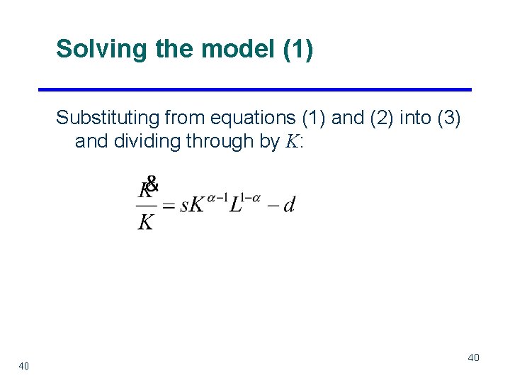
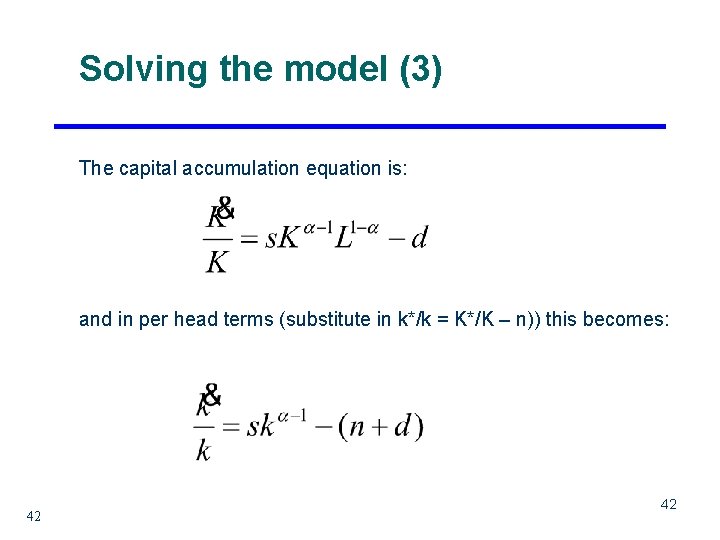
Solving the model (1) Substituting from equations (1) and (2) into (3) and dividing through by K: 40 40

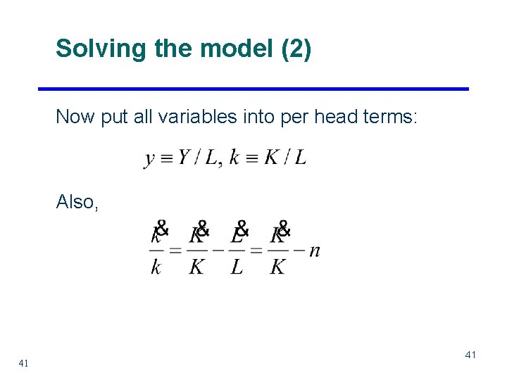
Solving the model (2) Now put all variables into per head terms: Also, 41 41

Solving the model (3) The capital accumulation equation is: and in per head terms (substitute in k*/k = K*/K – n)) this becomes: 42 42

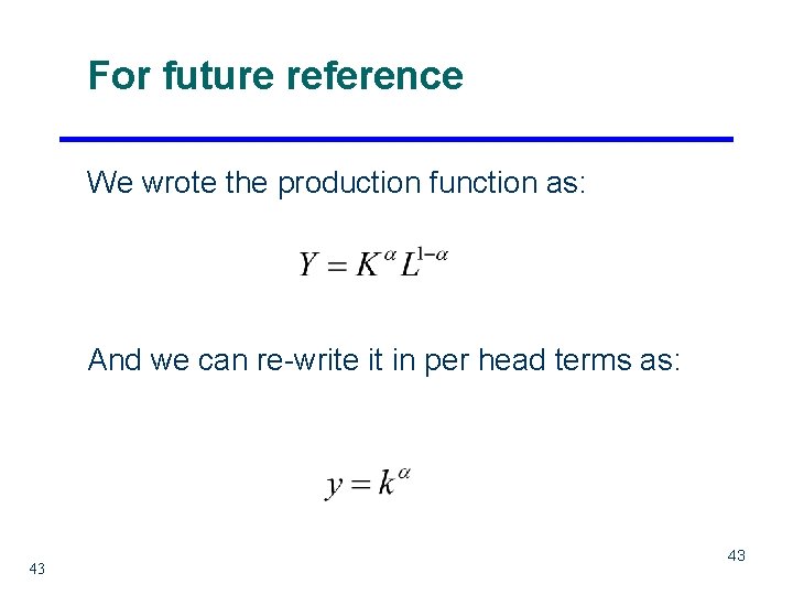
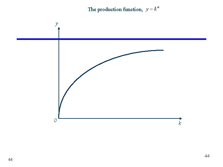
For future reference We wrote the production function as: And we can re-write it in per head terms as: 43 43

The production function, y 0 44 k 44

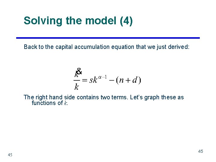
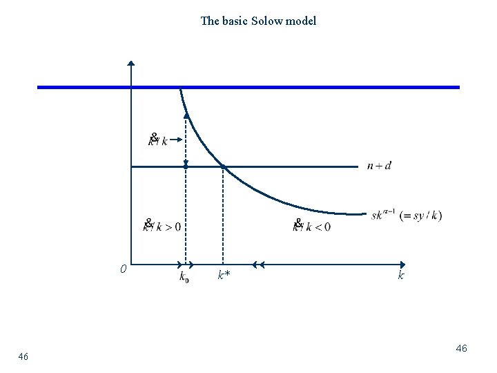
Solving the model (4) Back to the capital accumulation equation that we just derived: The right hand side contains two terms. Let’s graph these as functions of k. 45 45

The basic Solow model 0 46 k* k 46

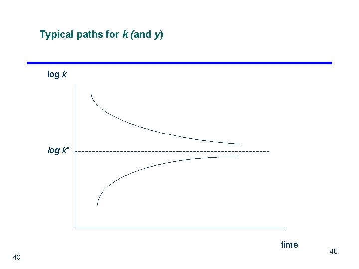
Conclusions of the basic Solow model l 47 The only possible equilibrium is one where output per head and capital per head (y and k) are constant. This equilibrium is stable --- if output and capital per head are initially above (below) the equilibrium levels, then they will fall (rise) till they are at these equilibrium levels. The long run (equilibrium) growth rate is zero. 47

Typical paths for k (and y) log k* time 48 48

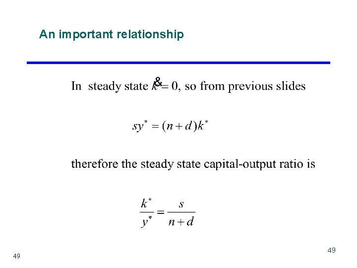
An important relationship 49 49

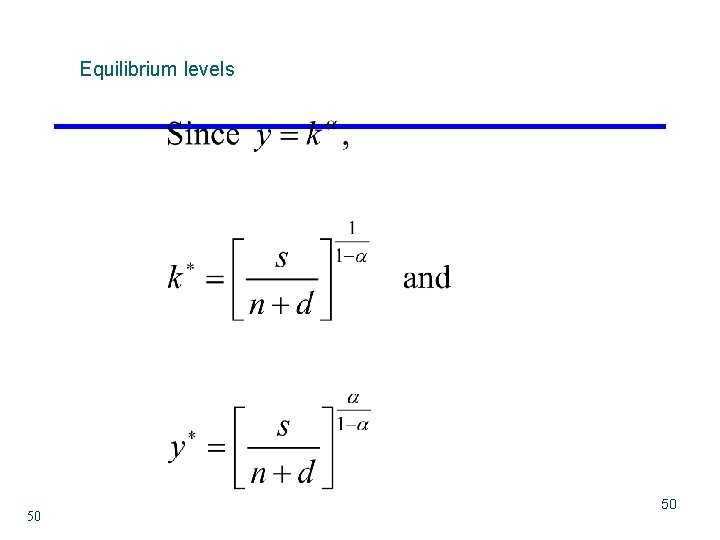
Equilibrium levels 50 50

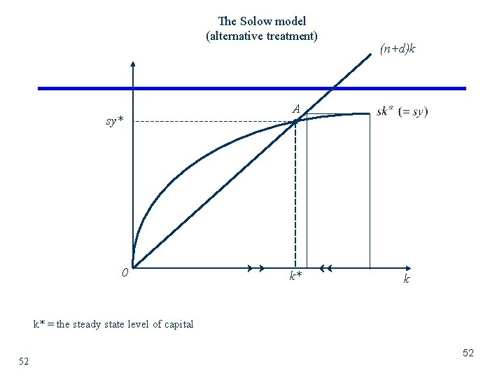
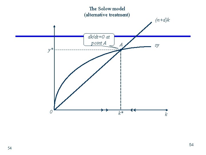
Alternative treatment Take the capital accumulation equation: Multiply through by k: Now graph the two terms on the right hand side as functions of k: 51 51

The Solow model (alternative treatment) sy* 0 (n+d)k A k* k k* = the steady state level of capital 52 52

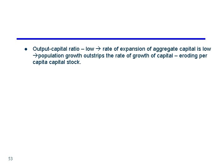
l 53 Output-capital ratio – low rate of expansion of aggregate capital is low population growth outstrips the rate of growth of capital – eroding per capital stock.

The Solow model (alternative treatment) dk/dt=0 at point A y* 0 54 A k* (n+d)k sy k 54

Solow and Growth Rates… l l 55 We wanted a growth model, but the solution shows that in the long run the growth rate is zero --- output per head and capital per head approach a constant level (y* and k*). For continuous per capita growth, capital must grow faster than population however, diminishing returns implies that the marginal contribution of capital to output declines decline in growth rate of output… l To get long run growth, we must have a motor of growth. In the Solow model this is exogenous technical progress l …optimistic force of continuing technical progress has to outweigh the doom of diminishing returns indefinite economic growth l Relative growth rates observed (in the context of this model) have to be transitional – i. e. occur during the transition to the steady state. (…. can be shown that faster growth occurs if a country is further away from its steady state…)

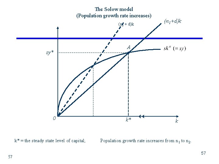
Population Growth in the Solow Model l 56 Quantity of capital available per worker decreases with population growth capital dilution.

The Solow model (Population growth rate increases) (n 2 + d)k sy* 0 k* = the steady state level of capital; 57 (n 1+d)k A k* k Population growth rate increases from n 1 to n 2. 57

The Solow Model: Income Differences – why are some countries rich and others poor? l l Differences in Investment Rates across countries: [yi*/yj*]= (si/sj)α/(1 -α) Higher investment rates translate into correspondingly higher levels of income across countries. l Why do investment rates across countries then…. ? ? l Savings rates perhaps? Differences in savings rates may arise for reasons unrelated to their levels of income per capita – Govt. policy/ income inequality/culture…. Savings rate may be affected by income itself (i. e. endogenous). (i) 58 Solow model regardless of the initial per capital stock, two countries with similar savings rates, depreciation rates and population growth rates will converge to similar standards of living in the long run

Government and Growth: A First Take 59 l Govt. policy affects the accumulation of physical capital l Govt policy and population growth… l Government encourages human capital formation l Tech… l Govt policy affects EFFICIENCY…

60 l Govt and the RULE of LAW. l Taxation, Efficiency & the Size of Govt. l Why do Govts do things that are bad for economic growth?

Long Run Growth and Institutions: the Argument l l Institutions---organization of society, “rules of the game”--- are a major determinant of economic performance and a key factor in understanding the vast cross-country differences in prosperity. Institutions are not exogenous, but there are potential sources of exogenous variation in history. – l 61 . Institutions are not typically chosen for the good of society, but imposed by groups with political power for their economic consequences.

Plan of the lectures (1) l Lecture 1: Institutional Causes of Economic Performance. – – – – – 62 Sources of prosperity. What are institutions? Brief discussion. Sources of cross-country differences in prosperity. Geography versus institutions and the identification problem. Learning from the Korean experiment. The colonial experiment and the Reversal of Fortune. Reassessing geography versus institutions. Are British colonies different? The role of culture.

Plan of the lectures (2) l Lecture 2: Towards a Theory of Institutions. – – – Different meta-theories: efficiency, history, ideology and social conflict. Economic institutions, political institutions and political power Historical examples: 1. 2. 3. – – – Dynamics of political power and political institutions. A theory of institutions. Historical examples: 1. 2. 63 Land relations in the Dutch East Indies Early financial development in the U. S. and Mexico Price regulation in Ghana, Kenya and Colombia Atlantic trade and rise of constitutional regimes. Emergence of mass democracy in Western Europe.

Sources of prosperity (1) 64 l Vast differences in prosperity across countries today. l Why? l Standard economic answers:

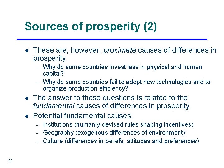
Sources of prosperity (2) l These are, however, proximate causes of differences in prosperity. – – l l The answer to these questions is related to the fundamental causes of differences in prosperity. Potential fundamental causes: – – – 65 Why do some countries invest less in physical and human capital? Why do some countries fail to adopt new technologies and to organize production efficiency? Institutions (humanly-devised rules shaping incentives) Geography (exogenous differences of environment) Culture (differences in beliefs, attitudes and preferences)

What are institutions? (1) l Institutions: the rules of the game in economic, political and social interactions. – l l North (1990, p. 3): "Institutions are the rules of the game in a society or, more formally, are the humanly devised constraints that shape human interaction. “ Key point: institutions – – – 66 Institutions determine “social organization” are humanly devised set constraints shape incentives

What are institutions? (2) l A broad cluster including many sub levels: – – l economic institutions: e. g. , property rights, contract enforcement, etc. l shape economic incentives, contracting possibilities, distribution. political institutions: e. g. , form of gov. , constraints on politicians and elites, separation of powers, etc. l shape political incentives and distribution of political power. Important distinction between: – Formal institutions: codified rules, e. g. in the constitution – Informal institutions: related to how formal institutions are used, to distribution of power, social norms, and equilibrium. l l 67 Constitutions in U. S. and many Latin American countries similar, but the practice of politics, and constraints on presidents and elites very different. Why? Because distribution of political power can be very different even when formal institutions are similar.