JPEG Still Image Data Compression Standard School of

JPEG Still Image Data Compression Standard School of Computer Science, University of Central Florida, VLSI and M-5 Research Group May, 1999

JPEG Introduction - The background n n JPEG stands for Joint Photographic Expert Group A standard image compression method is needed to enable interoperability of equipment from different manufacturer It is the first international digital image compression standard for continuous-tone images (grayscale or color) The history of JPEG – the selection process

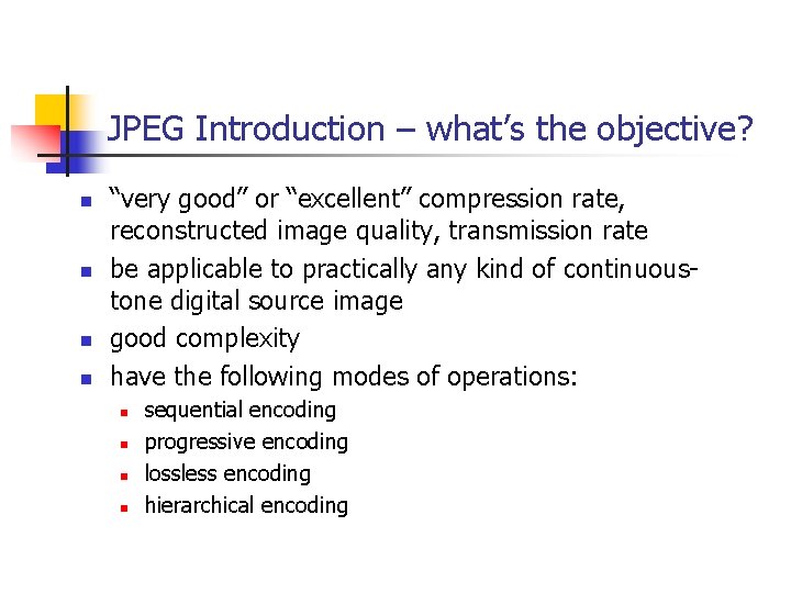
JPEG Introduction – what’s the objective? n n “very good” or “excellent” compression rate, reconstructed image quality, transmission rate be applicable to practically any kind of continuoustone digital source image good complexity have the following modes of operations: n n sequential encoding progressive encoding lossless encoding hierarchical encoding

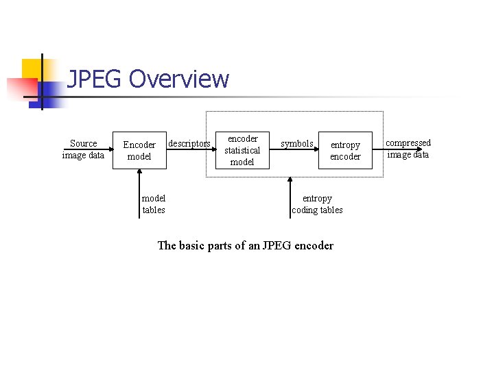
JPEG Overview Source image data descriptors Encoder model tables encoder statistical model symbols entropy encoder entropy coding tables The basic parts of an JPEG encoder compressed image data

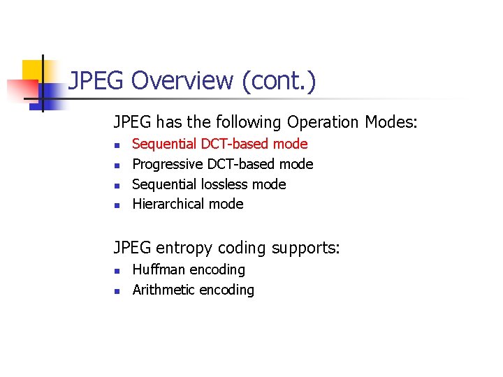
JPEG Overview (cont. ) JPEG has the following Operation Modes: n n Sequential DCT-based mode Progressive DCT-based mode Sequential lossless mode Hierarchical mode JPEG entropy coding supports: n n Huffman encoding Arithmetic encoding

JPEG Baseline System

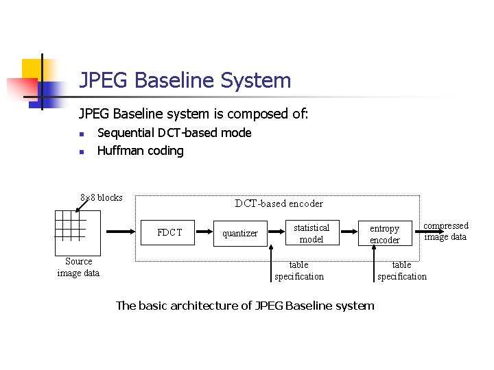
JPEG Baseline System JPEG Baseline system is composed of: n n Sequential DCT-based mode Huffman coding 8 8 blocks DCT-based encoder FDCT Source image data quantizer statistical model entropy encoder table specification The basic architecture of JPEG Baseline system compressed image data table specification

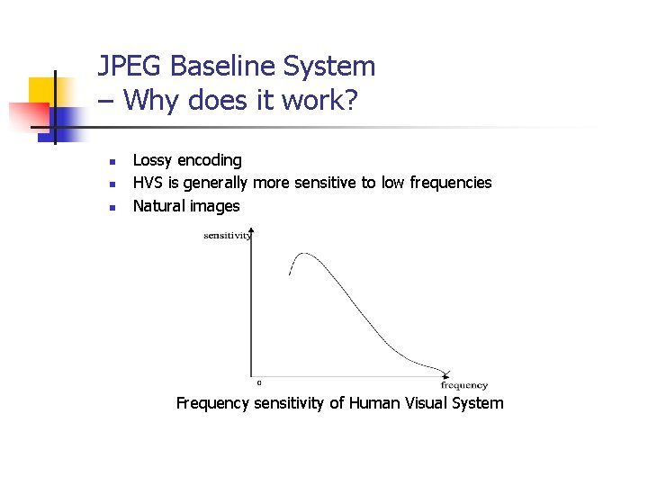
JPEG Baseline System – Why does it work? n n n Lossy encoding HVS is generally more sensitive to low frequencies Natural images Frequency sensitivity of Human Visual System

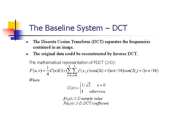
The Baseline System – DCT n n The Discrete Cosine Transform (DCT) separates the frequencies contained in an image. The original data could be reconstructed by Inverse DCT. The mathematical representation of FDCT (2 -D): Where f(x, y): 2 -D sample value F(u, v): 2 -D DCT coefficient

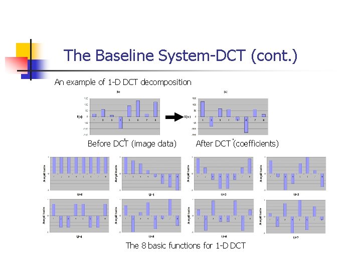
The Baseline System-DCT (cont. ) An example of 1 -D DCT decomposition Before DCT (image data) After DCT (coefficients) The 8 basic functions for 1 -D DCT

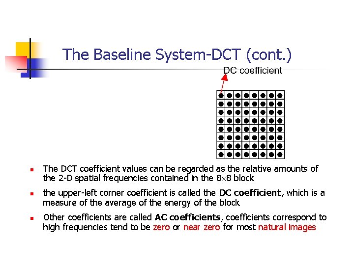
The Baseline System-DCT (cont. ) n n n The DCT coefficient values can be regarded as the relative amounts of the 2 -D spatial frequencies contained in the 8 8 block the upper-left corner coefficient is called the DC coefficient, which is a measure of the average of the energy of the block Other coefficients are called AC coefficients, coefficients correspond to high frequencies tend to be zero or near zero for most natural images

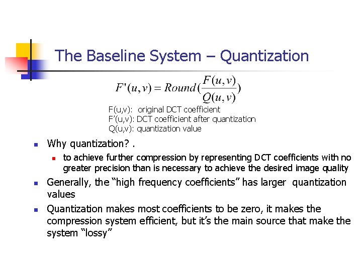
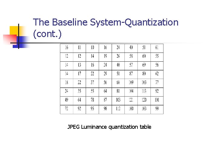
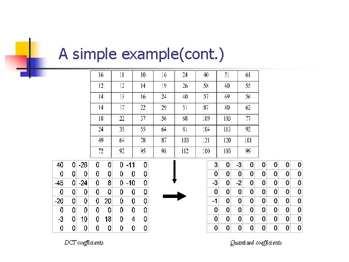
The Baseline System – Quantization F(u, v): original DCT coefficient F’(u, v): DCT coefficient after quantization Q(u, v): quantization value n Why quantization? . n n n to achieve further compression by representing DCT coefficients with no greater precision than is necessary to achieve the desired image quality Generally, the “high frequency coefficients” has larger quantization values Quantization makes most coefficients to be zero, it makes the compression system efficient, but it’s the main source that make the system “lossy”

The Baseline System-Quantization (cont. ) JPEG Luminance quantization table

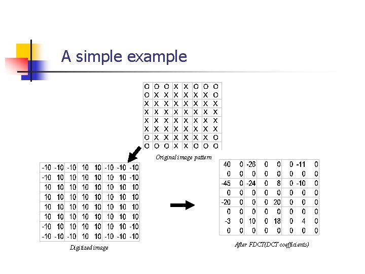
A simple example Original image pattern Digitized image After FDCT(DCT coefficients)

A simple example(cont. ) DCT coefficients Quantized coefficients

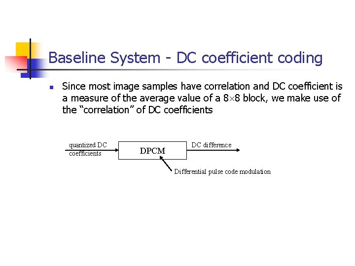
Baseline System - DC coefficient coding n Since most image samples have correlation and DC coefficient is a measure of the average value of a 8 8 block, we make use of the “correlation” of DC coefficients quantized DC coefficients DPCM DC difference Differential pulse code modulation

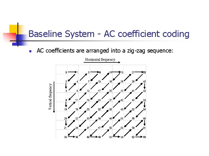
Baseline System - AC coefficient coding AC coefficients are arranged into a zig-zag sequence: Horizontal frequency Vertical frequency n

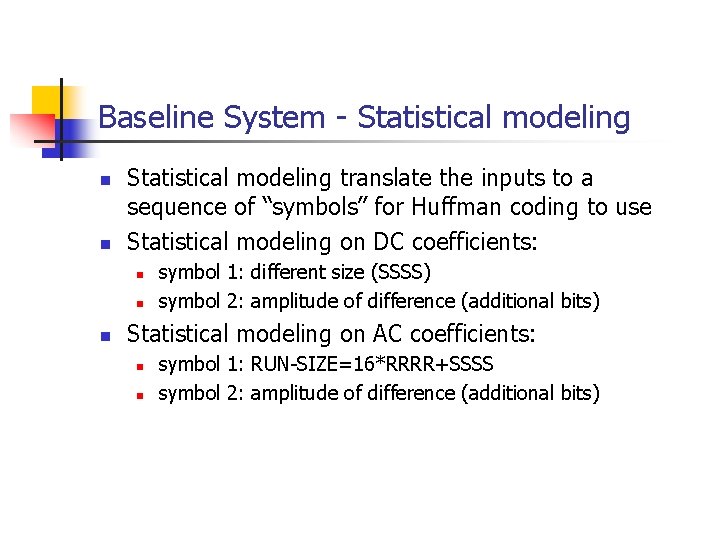
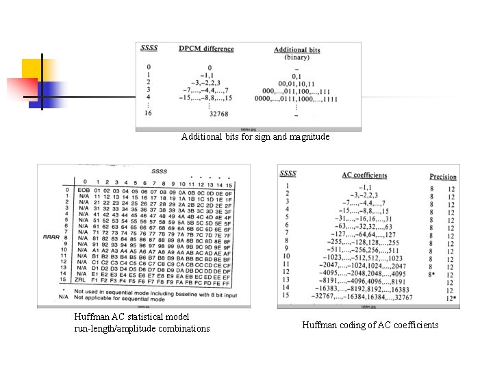
Baseline System - Statistical modeling n n Statistical modeling translate the inputs to a sequence of “symbols” for Huffman coding to use Statistical modeling on DC coefficients: n n n symbol 1: different size (SSSS) symbol 2: amplitude of difference (additional bits) Statistical modeling on AC coefficients: n n symbol 1: RUN-SIZE=16*RRRR+SSSS symbol 2: amplitude of difference (additional bits)

Additional bits for sign and magnitude Huffman AC statistical model run-length/amplitude combinations Huffman coding of AC coefficients

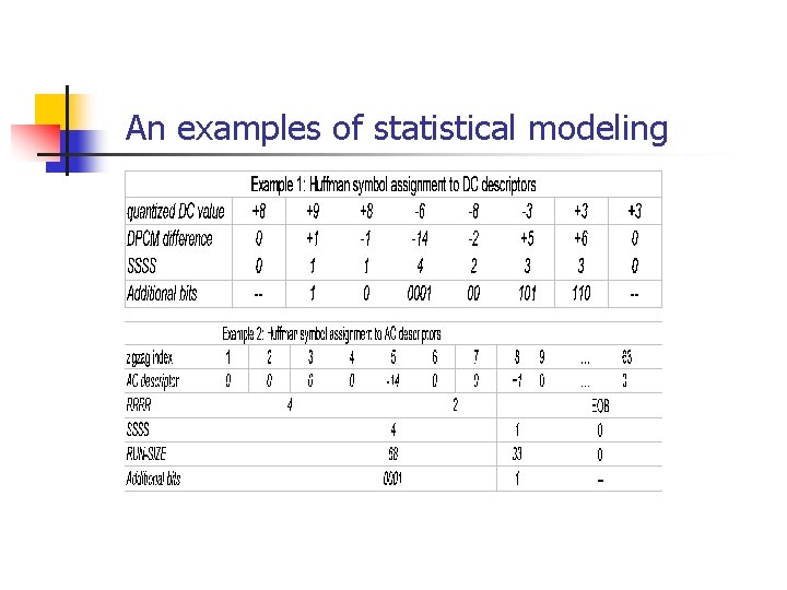
An examples of statistical modeling

Other Operation Modes

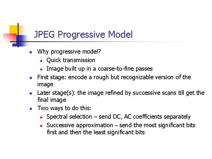
JPEG Progressive Model n n Why progressive model? n Quick transmission n Image built up in a coarse-to-fine passes First stage: encode a rough but recognizable version of the image Later stage(s): the image refined by successive scans till get the final image Two ways to do this: n Spectral selection – send DC, AC coefficients separately n Successive approximation – send the most significant bits first and then the least significant bits

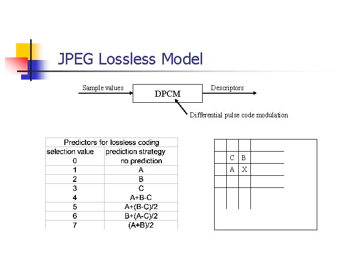
JPEG Lossless Model Sample values DPCM Descriptors Differential pulse code modulation C B A X

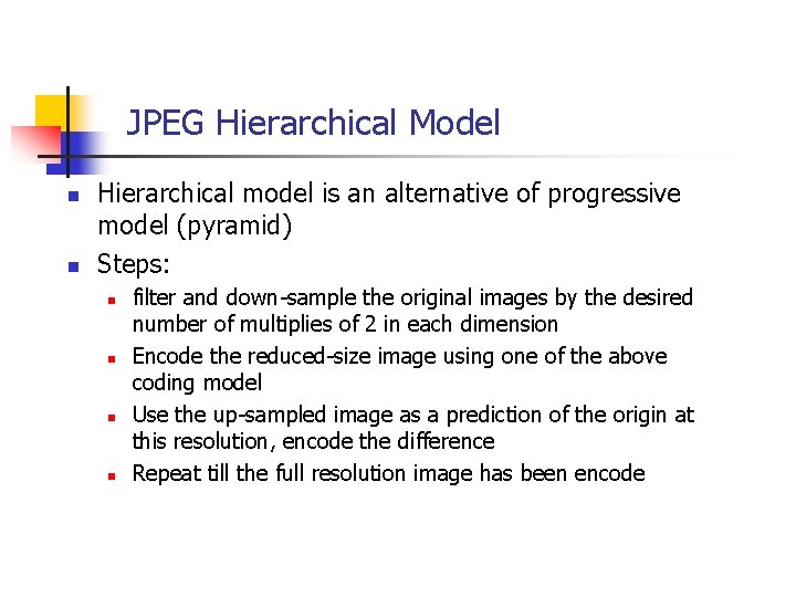
JPEG Hierarchical Model n n Hierarchical model is an alternative of progressive model (pyramid) Steps: n n filter and down-sample the original images by the desired number of multiplies of 2 in each dimension Encode the reduced-size image using one of the above coding model Use the up-sampled image as a prediction of the origin at this resolution, encode the difference Repeat till the full resolution image has been encode