Short Run Long Run Equilibrium Under Perfect Competition

Short Run Equilibrium In Perfectly Competitive Markets u Given: – – u Market Demand Firms’ Technologies (including some fixed inputs) Factor Prices The Number of Firms Need: – Each firm is profit maximizing – Market Demand = Short Run Market Supply u Solve For: – – P Q q profit

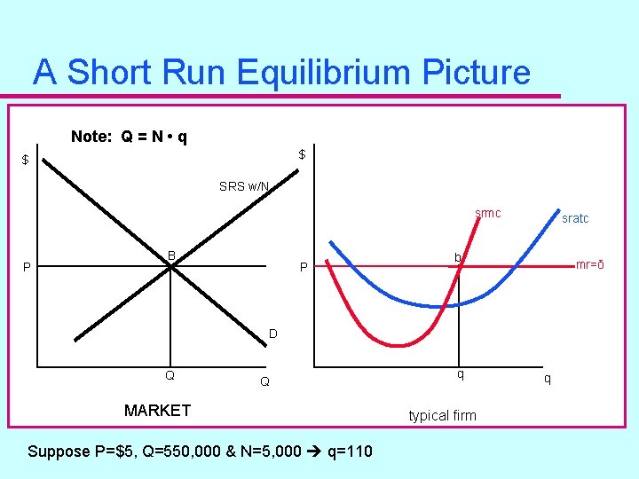
A Short Run Equilibrium Picture Note: Q = N • q $ $ SRS w/N srmc P B P sratc b mr=δ D Q Q MARKET Suppose P=$5, Q=550, 000 & N=5, 000 q=110 q typical firm q

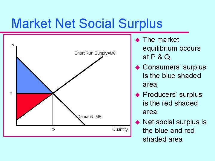
Market Net Social Surplus u P Short Run Supply=MC u P u Demand=MB u Q Quantity The market equilibrium occurs at P & Q. Consumers’ surplus is the blue shaded area Producers’ surplus is the red shaded area Net social surplus is the blue and red shaded area

Long Run Equilibrium In Perfectly Competitive Markets u All the short run equilibrium properties hold. u But also add… no firms wish to exit the market nor do firms want to enter. u Get: (P*, Q*, q*, N*) u Note: For there to be neither entry or exit, need economic profit to be zero. This is a long run equilibrium requirement. Otherwise the number of firms in the market will still be in flux. – Short run profit invites entry. – Short run losses suggest exit. – If firms ARE NOT identical, then it’s really that the marginal firm has zero profit.

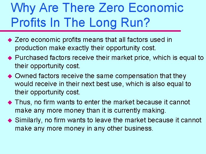
Why Are There Zero Economic Profits In The Long Run? u u u Zero economic profits means that all factors used in production make exactly their opportunity cost. Purchased factors receive their market price, which is equal to their opportunity cost. Owned factors receive the same compensation that they would receive in their next best use, which is also equal to their opportunity cost. Thus, no firm wants to enter the market because it cannot make any more money than it is currently making. Similarly, no firm wants to leave the market because it cannot make any more money in any other business.

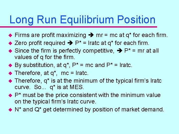
Long Run Equilibrium Position u u u u Firms are profit maximizing mr = mc at q* for each firm. Zero profit required P* = lratc at q* for each firm. Since the firm is perfectly competitive, P* = mr at all values of q for the firm. By substitution, at q*, P* = mc and P* = lratc. Therefore, at q*, mc = lratc. Therefore, q* is at the minimum of the typical firm’s lratc curve. So. . . q* is at MES. P* must be the price consistent with the minimum value on the typical firm’s lratc curve. N* and Q* get determined by position of market demand.

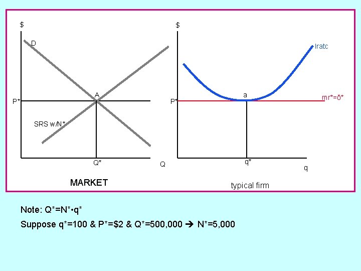
$ $ D lratc A P* a P* mr*=δ* SRS w/N* Q* MARKET q* Q typical firm Note: Q*=N* • q* Suppose q*=100 & P*=$2 & Q*=500, 000 N*=5, 000 q

Steps to Draw The Picture? u Doesn’t matter how you draw it, as long as you draw it correctly in the end. u Draw-a-person test.

What’s not ok. . .

Long Run Firm Supply u Never really use it, so no one bothers to really talk about it too much. u Could get it, but, let’s move on…

Long Run Market Supply u The long run market supply curve measures the quantities of a good or service offered for sale by all sellers--potential and actual--who could sell in the market. u The long run market supply curve represents the market relationship between P* and Q* when the market is in long run equilibrium.

Getting The Long Run Market Supply Curve (Suppose An Increases In Demand) u When demand increases and is expected to remain at the increased level, the short run response is to move along the short run supply curve--higher price and greater quantity supplied. u The long run response is to have entry in the market, movement along the long run supply curve--price returns to the minimum average total cost and quantity supplied increases.

$ sratc $ D 1 D 0 lratc srmc B b P’ P’ C A P* P* mr’=δ’ a mr*=δ* SRS 0 w/N* SRS 1 w/N** Q* Q’ Q** Q q* q’ q** MARKET q typical firm Note: Q*=N* • q*, Q’=N* • q’, Q**=N** • q** and q**=q* Suppose q*=100, P*=$2 & Q*=500, 000 N*=5, 000 Suppose P’=$5 & Q’=550, 000 q’=Q’/N*=110 Suppose Q**=600, 000 N**=6, 000 since P**=P*=$2 and q**=q*=100 and N**=Q**/q**

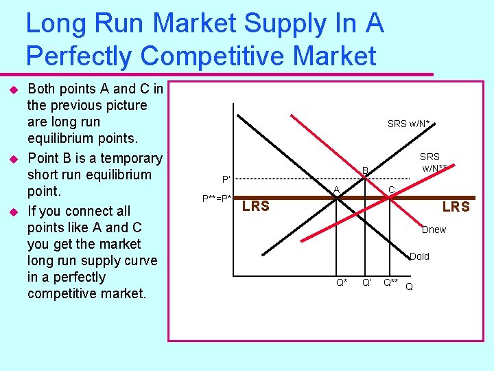
Long Run Market Supply In A Perfectly Competitive Market u u u Both points A and C in the previous picture are long run equilibrium points. Point B is a temporary short run equilibrium point. If you connect all points like A and C you get the market long run supply curve in a perfectly competitive market. SRS w/N* B P’ P**=P* SRS w/N** A C LRS Dnew Dold Q* Q’ Q** Q

Long Run Market Supply In A Perfectly Competitive Market u u The long run supply curve in the market is horizontal at the long run equilibrium price P*. P* is sometimes called the “normal price. ” P* is the price consistent with the typical firm’s minimum long run average total cost. Note: important assumption is that the position of the firm’s cost curve is unaffected by entry (or exit) of firms in the market. $ SRS w/N* SRSw/N** B P’ P**=P* A C LRS Dnew Dold Q* Q’ Q** Q

Short Run Versus Long Run Market Supply Curves: Recap u Along the short run market supply curve the number of firms in the industry is fixed, along with any fixed factors of production for the firm. u Along the long run market supply curve all firms operate at the point where marginal cost equals average cost. The number of firms adjusts to vary the supply. u Remember, all firms have been assumed to be identical. – What if that’s not the case? u Remember, an assumption of perfectly competitive markets is that firms can freely enter and exit.

A Note On: External Economies And Diseconomies Of Scale u If the industry exhibits no external economies or diseconomies of scale, then the industry long run supply curve is perfectly elastic (horizontal). The industry grows by replicating firms at the efficient scale. Entry and exit leaves the position of cost curves intact. This is often called a constant cost industry. u If the industry exhibits external diseconomies of scale, then the industry long run supply curve is upward sloping. The minimum average total cost of all firms in the industry rises as the size of the market grows (and falls as it contracts). This is often called an increasing cost industry. u If the industry exhibits external economies of scale, then the industry long run supply curve is downward sloping. The minimum average total cost falls as the size of the industry grows (and rises as it contracts). This is often called a decreasing cost industry.