Microsoft Excel 2016 Lesson 1 Overview 2016 John

Microsoft Excel 2016 Lesson 1 Overview © 2016, John Wiley & Sons, Inc. Microsoft Official Academic Course, Microsoft Excel Core 2016 1

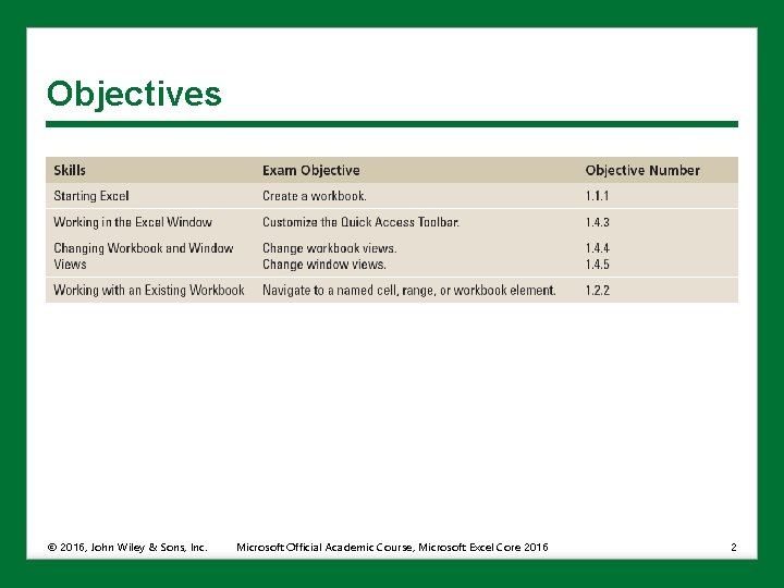
Objectives © 2016, John Wiley & Sons, Inc. Microsoft Official Academic Course, Microsoft Excel Core 2016 2

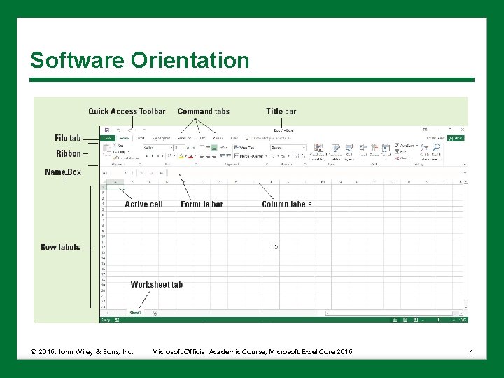
Software Orientation • Excel 2016 provides powerful tools to organize, analyze, manage, and share information. • The foundation of Excel and locations where you do your work are cells, rows, and columns within a worksheet, and worksheets as part of a workbook. • The tools you use while working in Excel are located on the ribbon across the top of the window. The ribbon is organized into task-oriented command tabs. • Each tab is divided into task-specific command groups with commands and options that relate to the group name. • You can customize the ribbon with new such as the Developer and Add-Ins tabs. The figure on the next slide shows the ribbon. © 2016, John Wiley & Sons, Inc. Microsoft Official Academic Course, Microsoft Excel Core 2016 3

Software Orientation © 2016, John Wiley & Sons, Inc. Microsoft Official Academic Course, Microsoft Excel Core 2016 4

Starting Excel • Click Start, All apps, and then Excel 2016 to open Excel. • Excel opens to a list of templates. • Typically, you will open a Blank workbook or open a previous file. • A workbook, or spreadsheet file, can be compared to a physical book with many pages. • When you open a blank workbook, the temporary filename (Book 1) and the program name (Excel) appear in the title bar at the top of the screen. • Book 1 (or Book 2, Book 3, and so on) is a temporary title for your workbook until you save the workbook with a name of your choice. © 2016, John Wiley & Sons, Inc. Microsoft Official Academic Course, Microsoft Excel Core 2016 5

Starting Excel • The new workbook contains one worksheet (Sheet 1) by default. • The sheet tabs are located just above the Status bar and are identified as Sheet 1, Sheet 2, and Sheet 3. (Think of these as pages. ) • Rename worksheets to identify their content. • Add worksheets with the New sheet (+) button as needed. © 2016, John Wiley & Sons, Inc. Microsoft Official Academic Course, Microsoft Excel Core 2016 6

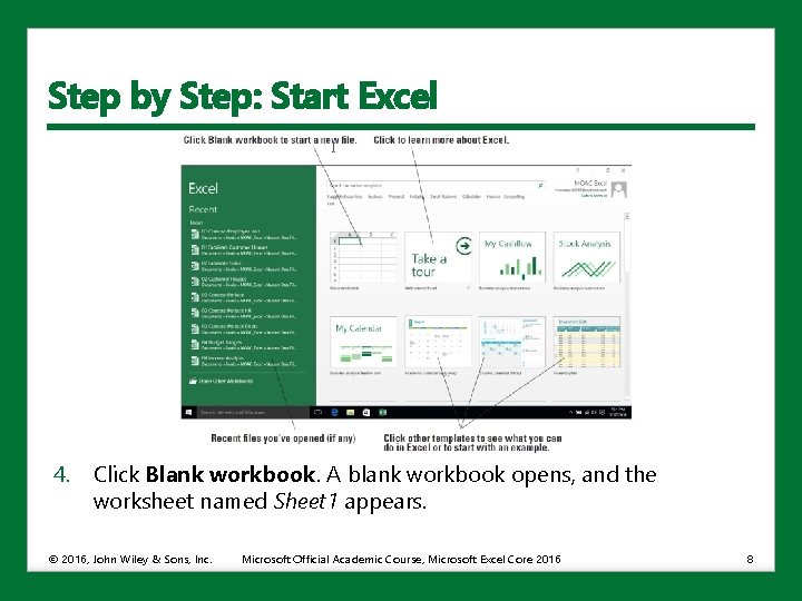
Step by Step: Start Excel • Be sure Microsoft Excel is installed on your computer. Then perform the following steps: 1. With the Windows desktop displayed, click the Start button in the lower-left corner of the Windows 10 screen. 2. Click All apps near the bottom of the Start menu. 3. In the list of applications, scroll down as necessary and click Excel 2016. The Excel window opens to display recent Excel files you’ve opened and examples of templates you can use (see the figure on the next slide). © 2016, John Wiley & Sons, Inc. Microsoft Official Academic Course, Microsoft Excel Core 2016 7

Step by Step: Start Excel 4. Click Blank workbook. A blank workbook opens, and the worksheet named Sheet 1 appears. © 2016, John Wiley & Sons, Inc. Microsoft Official Academic Course, Microsoft Excel Core 2016 8

Step by Step: Start Excel • A worksheet is a grid composed of rows, columns, and cells. • Each worksheet column starts at the top of the worksheet and goes to the bottom of the worksheet and is identified by a letter. • Each row starts at the left edge of the worksheet and continues to the right and is identified by a number. • Each box, or cell, on the grid is identified by the intersection of a column and a row. • Enter information by typing it into the active cell (also called the current or highlighted cell), which is outlined by a bold rectangle. © 2016, John Wiley & Sons, Inc. Microsoft Official Academic Course, Microsoft Excel Core 2016 9

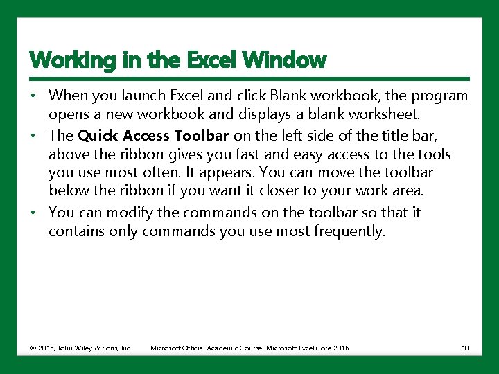
Working in the Excel Window • When you launch Excel and click Blank workbook, the program opens a new workbook and displays a blank worksheet. • The Quick Access Toolbar on the left side of the title bar, above the ribbon gives you fast and easy access to the tools you use most often. It appears. You can move the toolbar below the ribbon if you want it closer to your work area. • You can modify the commands on the toolbar so that it contains only commands you use most frequently. © 2016, John Wiley & Sons, Inc. Microsoft Official Academic Course, Microsoft Excel Core 2016 10

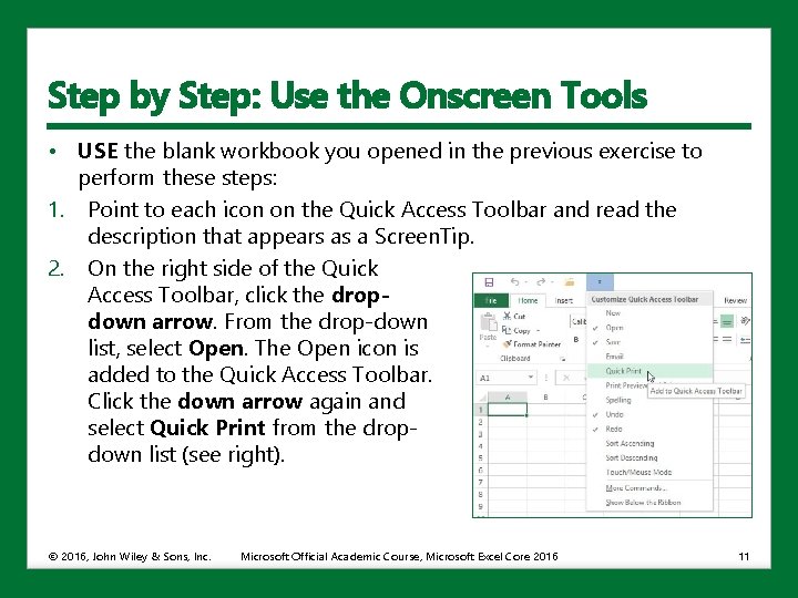
Step by Step: Use the Onscreen Tools • USE the blank workbook you opened in the previous exercise to perform these steps: 1. Point to each icon on the Quick Access Toolbar and read the description that appears as a Screen. Tip. 2. On the right side of the Quick Access Toolbar, click the dropdown arrow. From the drop-down list, select Open. The Open icon is added to the Quick Access Toolbar. Click the down arrow again and select Quick Print from the dropdown list (see right). © 2016, John Wiley & Sons, Inc. Microsoft Official Academic Course, Microsoft Excel Core 2016 11

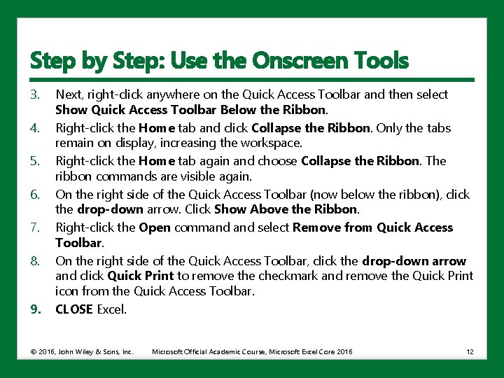
Step by Step: Use the Onscreen Tools 3. 4. 5. 6. 7. 8. 9. Next, right-click anywhere on the Quick Access Toolbar and then select Show Quick Access Toolbar Below the Ribbon. Right-click the Home tab and click Collapse the Ribbon. Only the tabs remain on display, increasing the workspace. Right-click the Home tab again and choose Collapse the Ribbon. The ribbon commands are visible again. On the right side of the Quick Access Toolbar (now below the ribbon), click the drop-down arrow. Click Show Above the Ribbon. Right-click the Open command select Remove from Quick Access Toolbar. On the right side of the Quick Access Toolbar, click the drop-down arrow and click Quick Print to remove the checkmark and remove the Quick Print icon from the Quick Access Toolbar. CLOSE Excel. © 2016, John Wiley & Sons, Inc. Microsoft Official Academic Course, Microsoft Excel Core 2016 12

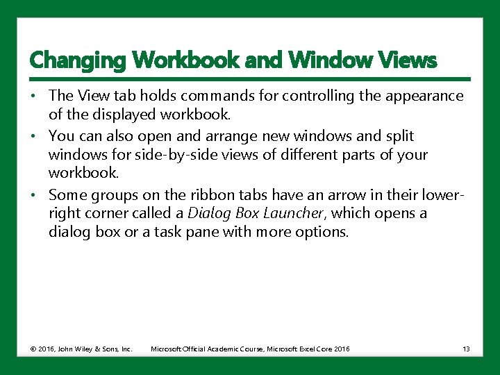
Changing Workbook and Window Views • The View tab holds commands for controlling the appearance of the displayed workbook. • You can also open and arrange new windows and split windows for side-by-side views of different parts of your workbook. • Some groups on the ribbon tabs have an arrow in their lowerright corner called a Dialog Box Launcher, which opens a dialog box or a task pane with more options. © 2016, John Wiley & Sons, Inc. Microsoft Official Academic Course, Microsoft Excel Core 2016 13

Step by Step: Change the Workbook View • LAUNCH Excel and start a new workbook. 1. If necessary, click the Home tab to activate it. 2. Select cell A 1 to make it active. Then type 456 and press Tab. 3. In the lower-right corner of the Font group, click the Dialog Box Launcher arrow. The Format Cells dialog box shown here opens. © 2016, John Wiley & Sons, Inc. Microsoft Official Academic Course, Microsoft Excel Core 2016 14

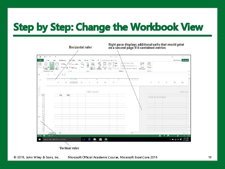
Step by Step: Change the Workbook View 4. Notice that the Font tab of the dialog box is active. Scroll down in the Font list, click Cambria, and then click OK. Cell B 1 is the active cell now. 5. Type 456 in this cell and then press Tab. Notice the difference in appearance between A 1 and B 1. 6. Click the View tab. 7. In the Workbook Views group, click Page Layout. In this view, you can see the margins, where pages break, and you can add a header or footer (see the figure on the next slide). 8. In the Workbook Views group, click Normal to return the worksheet to the Normal view. © 2016, John Wiley & Sons, Inc. Microsoft Official Academic Course, Microsoft Excel Core 2016 15

Step by Step: Change the Workbook View © 2016, John Wiley & Sons, Inc. Microsoft Official Academic Course, Microsoft Excel Core 2016 16

Splitting the Window • When a worksheet contains a lot of data, you can see only a small portion of the worksheet in Excel’s Normal and Page Layout views. • The Split command enables to view the worksheet in two panes or four quadrants. • The Split command lets you use the scroll bars on the right and at the bottom of the window to display different sections of the worksheet at the same time so you can compare or contrast data or see what effect a change in one part of the worksheet might have on a distant part of the worksheet. © 2016, John Wiley & Sons, Inc. Microsoft Official Academic Course, Microsoft Excel Core 2016 17

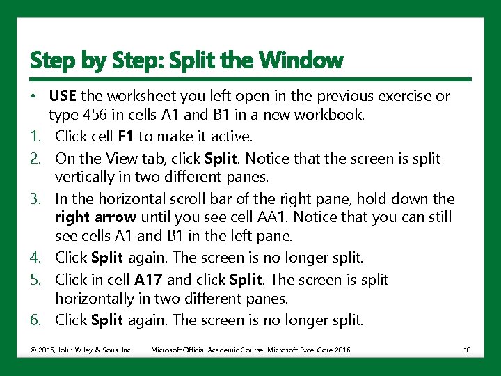
Step by Step: Split the Window • USE the worksheet you left open in the previous exercise or type 456 in cells A 1 and B 1 in a new workbook. 1. Click cell F 1 to make it active. 2. On the View tab, click Split. Notice that the screen is split vertically in two different panes. 3. In the horizontal scroll bar of the right pane, hold down the right arrow until you see cell AA 1. Notice that you can still see cells A 1 and B 1 in the left pane. 4. Click Split again. The screen is no longer split. 5. Click in cell A 17 and click Split. The screen is split horizontally in two different panes. 6. Click Split again. The screen is no longer split. © 2016, John Wiley & Sons, Inc. Microsoft Official Academic Course, Microsoft Excel Core 2016 18

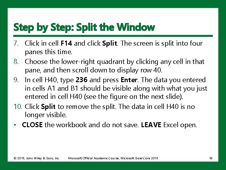
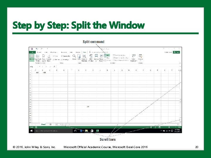
Step by Step: Split the Window 7. Click in cell F 14 and click Split. The screen is split into four panes this time. 8. Choose the lower-right quadrant by clicking any cell in that pane, and then scroll down to display row 40. 9. In cell H 40, type 236 and press Enter. The data you entered in cells A 1 and B 1 should be visible along with what you just entered in cell H 40 (see the figure on the next slide). 10. Click Split to remove the split. The data in cell H 40 is no longer visible. • CLOSE the workbook and do not save. LEAVE Excel open. © 2016, John Wiley & Sons, Inc. Microsoft Official Academic Course, Microsoft Excel Core 2016 19

Step by Step: Split the Window © 2016, John Wiley & Sons, Inc. Microsoft Official Academic Course, Microsoft Excel Core 2016 20

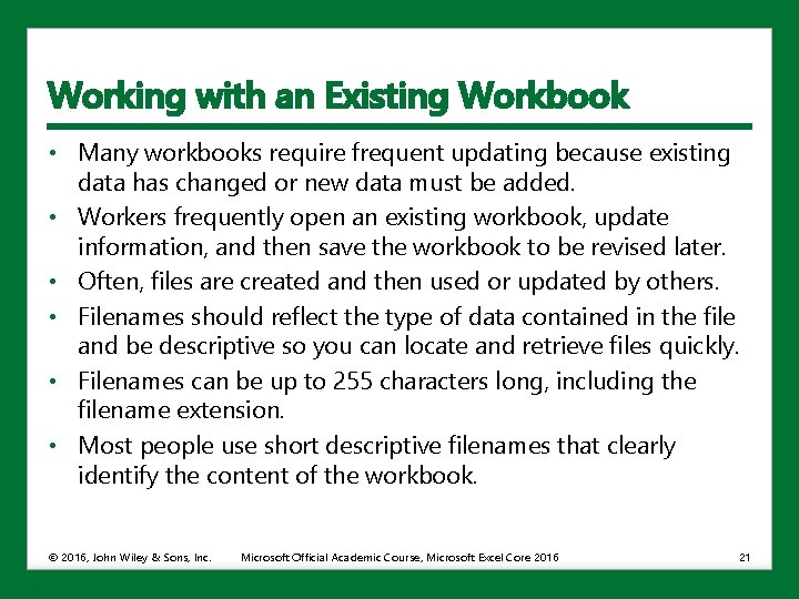
Working with an Existing Workbook • Many workbooks require frequent updating because existing data has changed or new data must be added. • Workers frequently open an existing workbook, update information, and then save the workbook to be revised later. • Often, files are created and then used or updated by others. • Filenames should reflect the type of data contained in the file and be descriptive so you can locate and retrieve files quickly. • Filenames can be up to 255 characters long, including the filename extension. • Most people use short descriptive filenames that clearly identify the content of the workbook. © 2016, John Wiley & Sons, Inc. Microsoft Official Academic Course, Microsoft Excel Core 2016 21

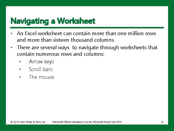
Navigating a Worksheet • An Excel worksheet can contain more than one million rows and more than sixteen thousand columns. • There are several ways to navigate through worksheets that contain numerous rows and columns: • Arrow keys • Scroll bars • The mouse © 2016, John Wiley & Sons, Inc. Microsoft Official Academic Course, Microsoft Excel Core 2016 22

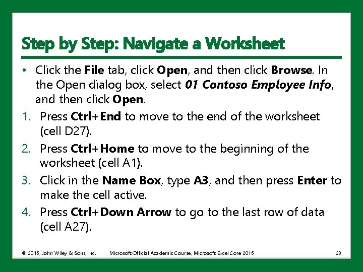
Step by Step: Navigate a Worksheet • Click the File tab, click Open, and then click Browse. In the Open dialog box, select 01 Contoso Employee Info, and then click Open. 1. Press Ctrl+End to move to the end of the worksheet (cell D 27). 2. Press Ctrl+Home to move to the beginning of the worksheet (cell A 1). 3. Click in the Name Box, type A 3, and then press Enter to make the cell active. 4. Press Ctrl+Down Arrow to go to the last row of data (cell A 27). © 2016, John Wiley & Sons, Inc. Microsoft Official Academic Course, Microsoft Excel Core 2016 23

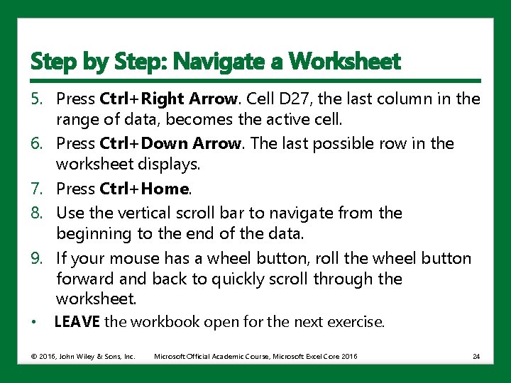
Step by Step: Navigate a Worksheet 5. Press Ctrl+Right Arrow. Cell D 27, the last column in the range of data, becomes the active cell. 6. Press Ctrl+Down Arrow. The last possible row in the worksheet displays. 7. Press Ctrl+Home. 8. Use the vertical scroll bar to navigate from the beginning to the end of the data. 9. If your mouse has a wheel button, roll the wheel button forward and back to quickly scroll through the worksheet. • LEAVE the workbook open for the next exercise. © 2016, John Wiley & Sons, Inc. Microsoft Official Academic Course, Microsoft Excel Core 2016 24

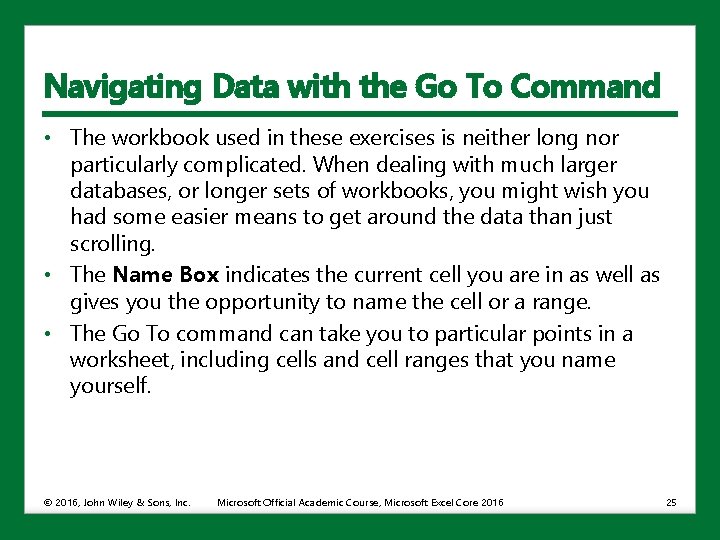
Navigating Data with the Go To Command • The workbook used in these exercises is neither long nor particularly complicated. When dealing with much larger databases, or longer sets of workbooks, you might wish you had some easier means to get around the data than just scrolling. • The Name Box indicates the current cell you are in as well as gives you the opportunity to name the cell or a range. • The Go To command can take you to particular points in a worksheet, including cells and cell ranges that you name yourself. © 2016, John Wiley & Sons, Inc. Microsoft Official Academic Course, Microsoft Excel Core 2016 25

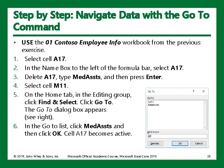
Step by Step: Navigate Data with the Go To Command • USE the 01 Contoso Employee Info workbook from the previous exercise. 1. Select cell A 17. 2. In the Name Box to the left of the formula bar, select A 17. 3. Delete A 17, type Med. Assts, and then press Enter. 4. Select cell M 11. 5. On the Home tab, in the Editing group, click Find & Select. Click Go To. The Go To dialog box appears (see right). 6. In the Go to list, click Med. Assts and then click OK. Cell A 17 becomes active. © 2016, John Wiley & Sons, Inc. Microsoft Official Academic Course, Microsoft Excel Core 2016 26

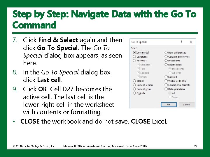
Step by Step: Navigate Data with the Go To Command 7. Click Find & Select again and then click Go To Special. The Go To Special dialog box appears, as seen here. 8. In the Go To Special dialog box, click Last cell. 9. Click OK. Cell D 27 becomes the active cell. The last cell is the lower-right cell in the worksheet with contents or formatting. • CLOSE the workbook and do not save. CLOSE Excel. © 2016, John Wiley & Sons, Inc. Microsoft Official Academic Course, Microsoft Excel Core 2016 27

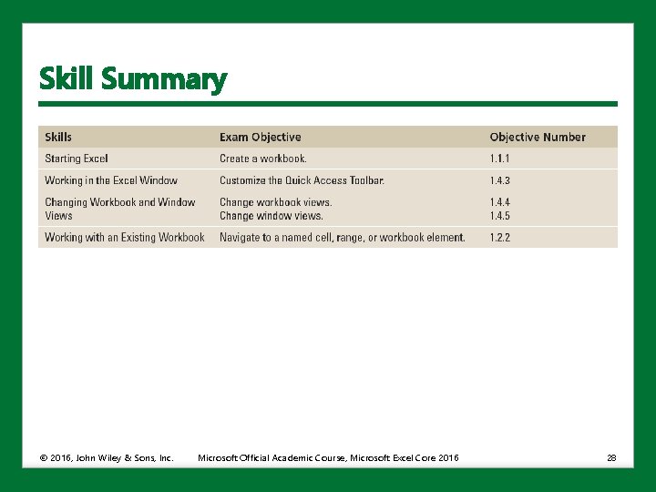
Skill Summary © 2016, John Wiley & Sons, Inc. Microsoft Official Academic Course, Microsoft Excel Core 2016 28