
Classification Outline a toolbox of useful algorithms concepts
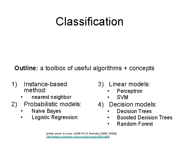
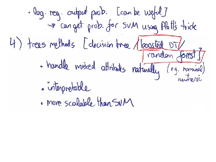
Classification Outline: a toolbox of useful algorithms + concepts 1) Instance-based method: • 2) nearest neighbor Probabilistic models: • • Naive Bayes Logistic Regression 3) Linear models: • • Perceptron SVM 4) Decision models: • • • [slides prises du cours cs 294 -10 UC Berkeley (2006 / 2009)] http: //www. cs. berkeley. edu/~jordan/courses/294 -fall 09 Decision Trees Boosted Decision Trees Random Forest
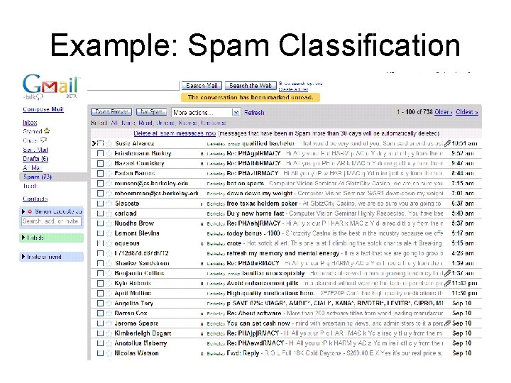
Example: Spam Classification
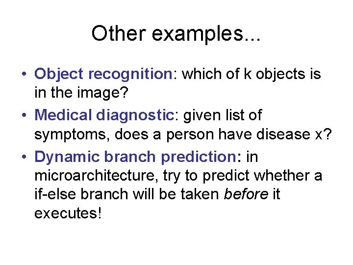
Other examples. . . • Object recognition: which of k objects is in the image? • Medical diagnostic: given list of symptoms, does a person have disease x? • Dynamic branch prediction: in microarchitecture, try to predict whether a if-else branch will be taken before it executes!
Setup
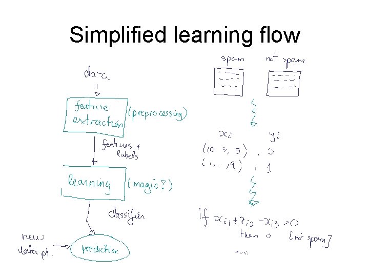
Simplified learning flow
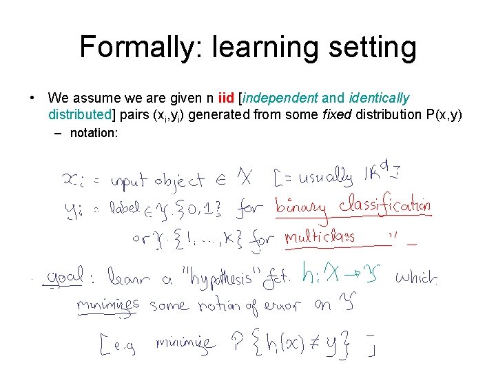
Formally: learning setting • We assume we are given n iid [independent and identically distributed] pairs (xi, yi) generated from some fixed distribution P(x, y) – notation:
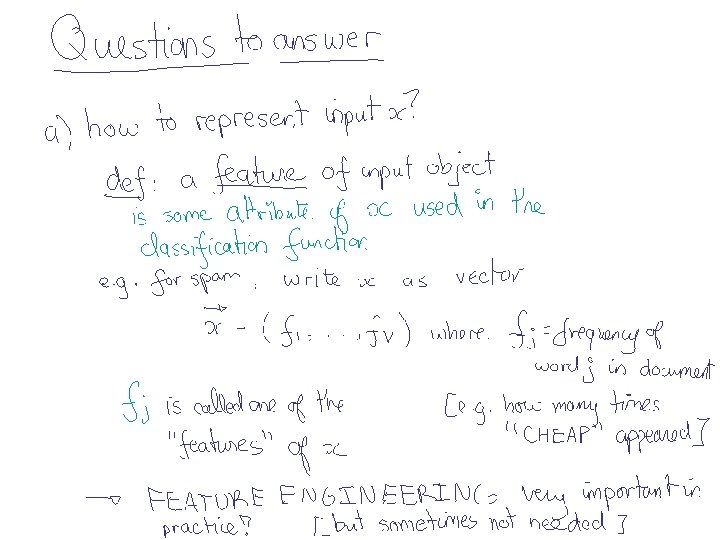
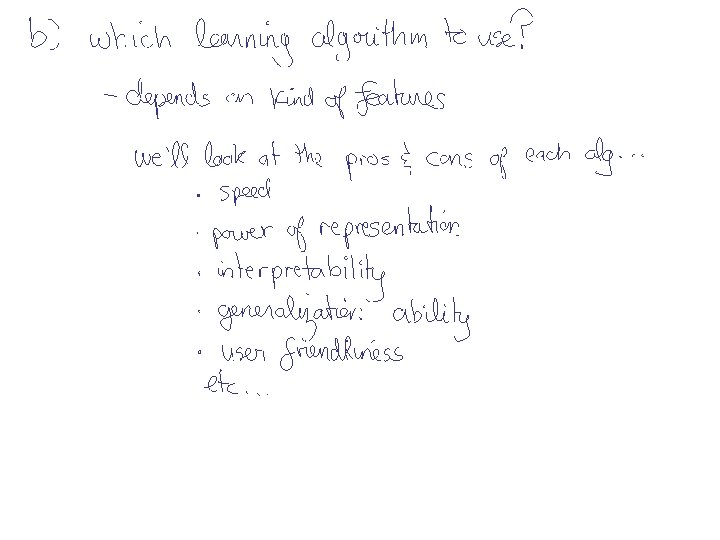
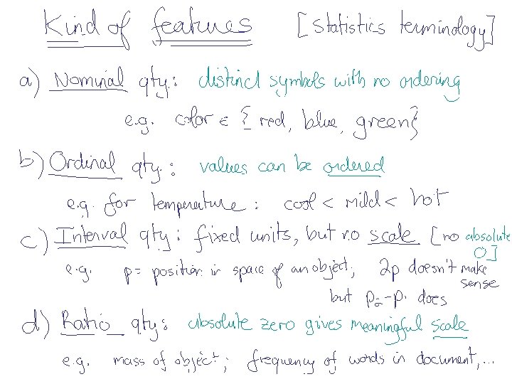
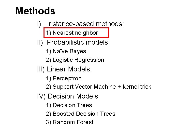
Methods I) Instance-based methods: 1) Nearest neighbor II) Probabilistic models: 1) Naïve Bayes 2) Logistic Regression III) Linear Models: 1) Perceptron 2) Support Vector Machine + kernel trick IV) Decision Models: 1) Decision Trees 2) Boosted Decision Trees 3) Random Forest
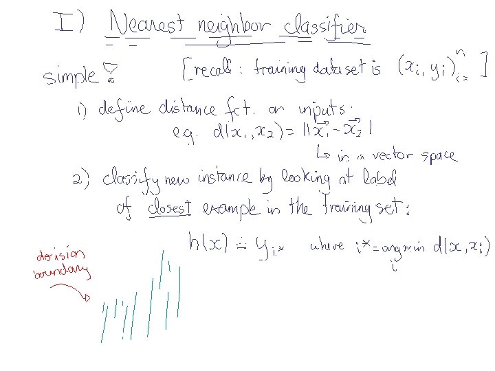
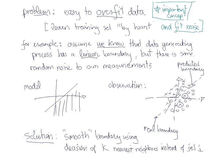
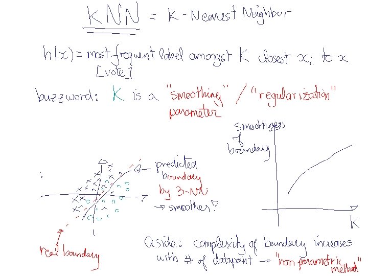
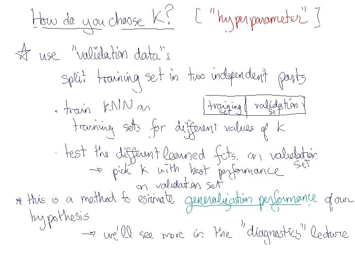
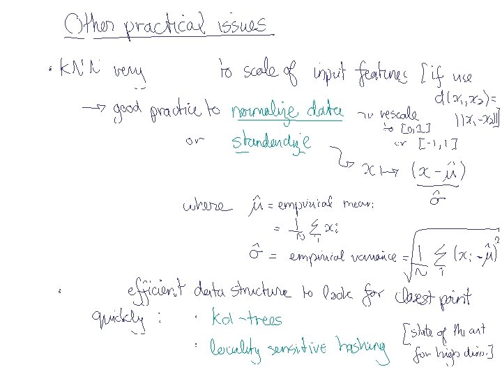
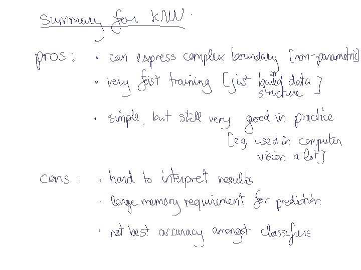
Methods I) Instance-based methods: 1) Nearest neighbor II) Probabilistic models: 1) Naïve Bayes 2) Logistic Regression III) Linear Models: 1) Perceptron 2) Support Vector Machine + kernel trick IV) Decision Models: 1) Decision Trees 2) Boosted Decision Trees 3) Random Forest
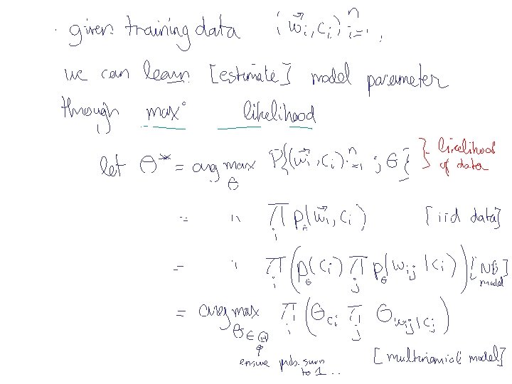
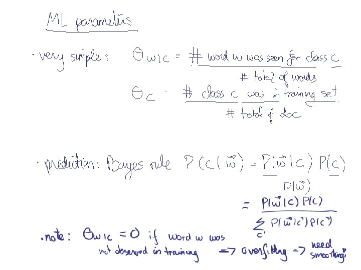
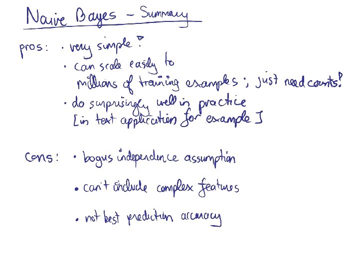
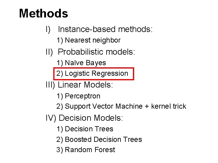
Methods I) Instance-based methods: 1) Nearest neighbor II) Probabilistic models: 1) Naïve Bayes 2) Logistic Regression III) Linear Models: 1) Perceptron 2) Support Vector Machine + kernel trick IV) Decision Models: 1) Decision Trees 2) Boosted Decision Trees 3) Random Forest
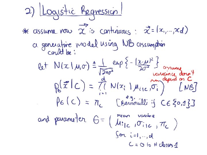
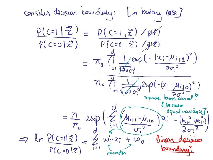
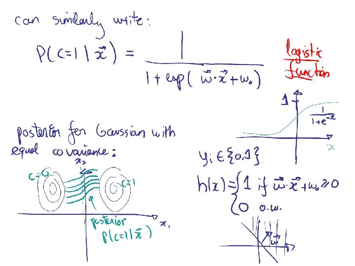
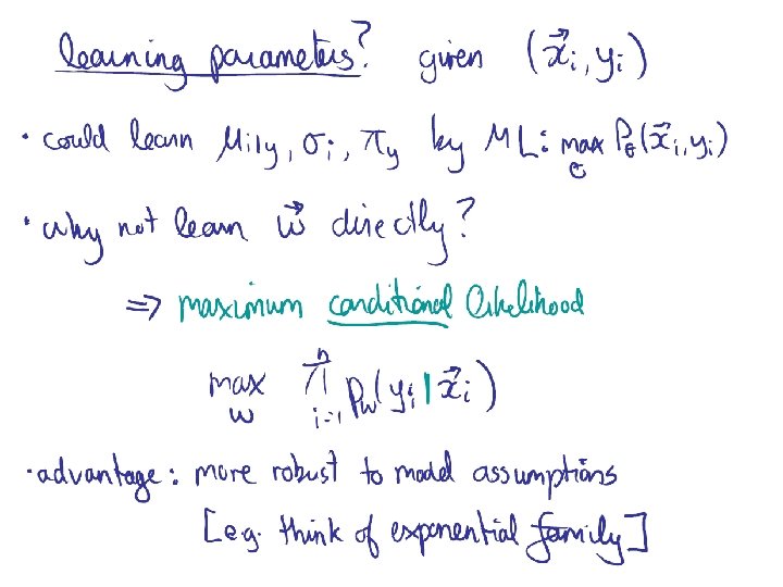
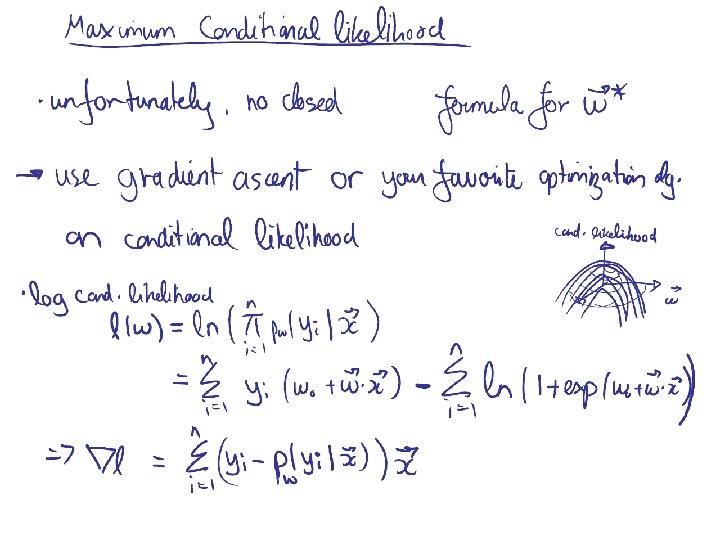
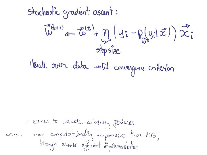
Methods I) Instance-based methods: 1) Nearest neighbor II) Probabilistic models: 1) Naïve Bayes 2) Logistic Regression III) Linear Models: 1) Perceptron 2) Support Vector Machine + kernel trick IV) Decision Models: 1) Decision Trees 2) Boosted Decision Trees 3) Random Forest
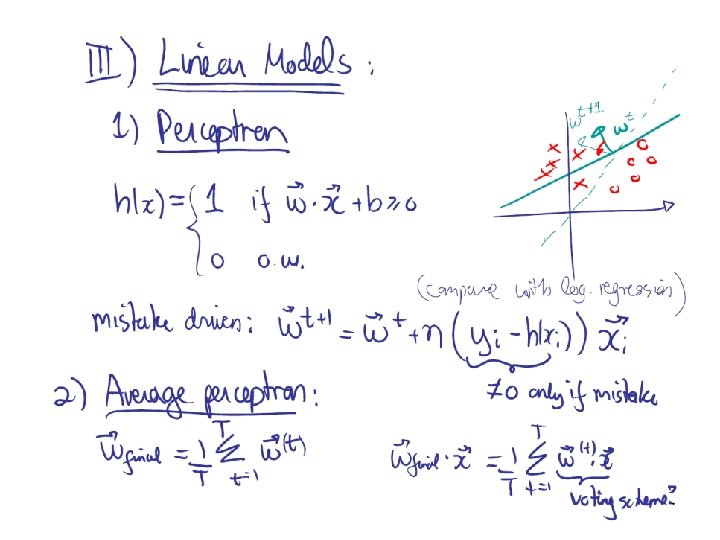
Methods I) Instance-based methods: 1) Nearest neighbor II) Probabilistic models: 1) Naïve Bayes 2) Logistic Regression III) Linear Models: 1) Perceptron 2) Support Vector Machine + kernel trick IV) Decision Models: 1) Decision Trees 2) Boosted Decision Trees 3) Random Forest
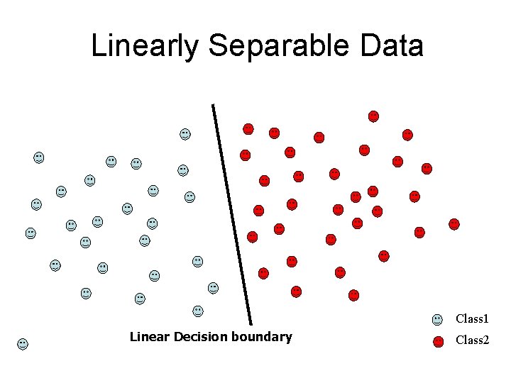
Linearly Separable Data Class 1 Linear Decision boundary Class 2
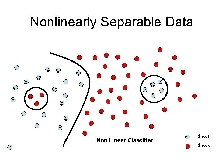
Nonlinearly Separable Data Non Linear Classifier Class 1 Class 2
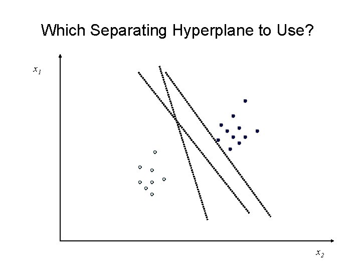
Which Separating Hyperplane to Use? x 1 x 2
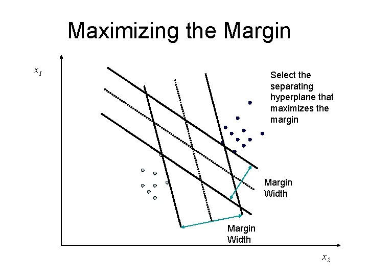
Maximizing the Margin x 1 Select the separating hyperplane that maximizes the margin Margin Width x 2
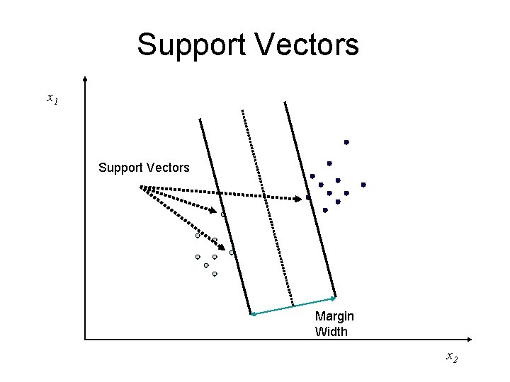
Support Vectors x 1 Support Vectors Margin Width x 2
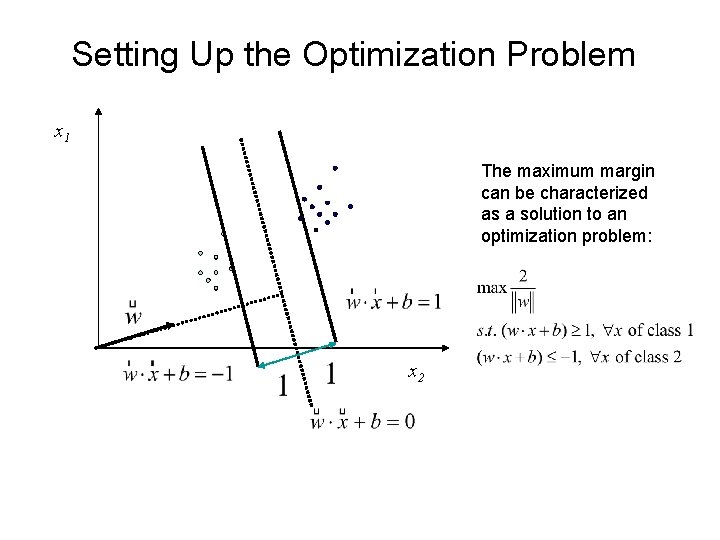
Setting Up the Optimization Problem x 1 The maximum margin can be characterized as a solution to an optimization problem: x 2
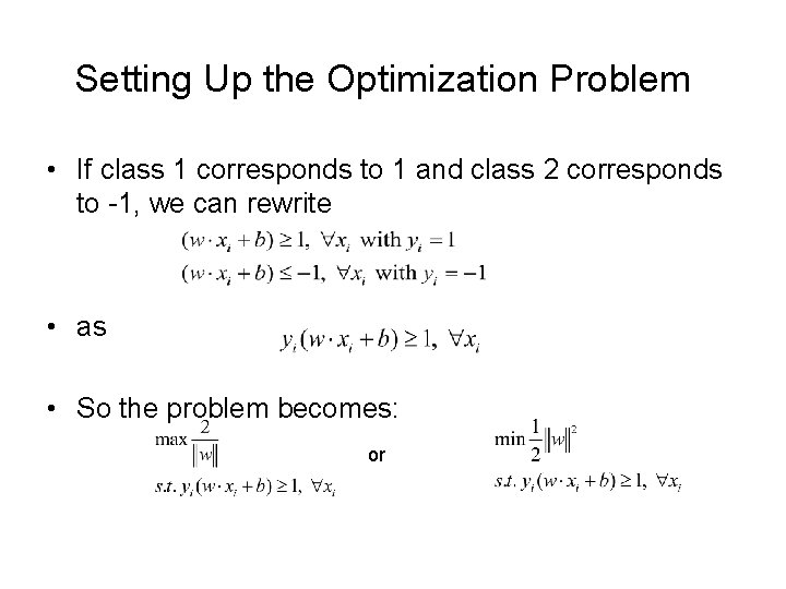
Setting Up the Optimization Problem • If class 1 corresponds to 1 and class 2 corresponds to -1, we can rewrite • as • So the problem becomes: or
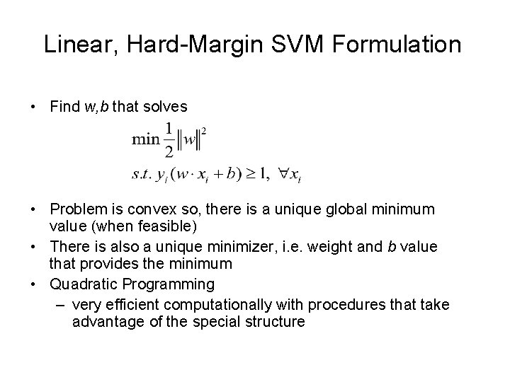
Linear, Hard-Margin SVM Formulation • Find w, b that solves • Problem is convex so, there is a unique global minimum value (when feasible) • There is also a unique minimizer, i. e. weight and b value that provides the minimum • Quadratic Programming – very efficient computationally with procedures that take advantage of the special structure
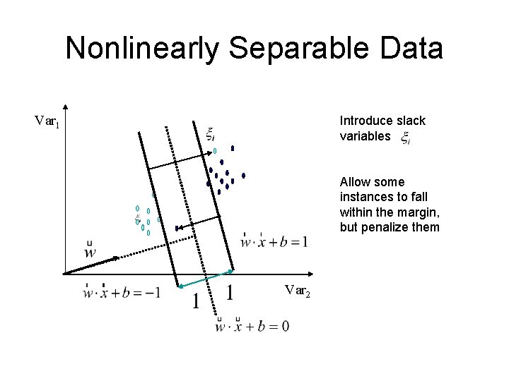
Nonlinearly Separable Data Var 1 Introduce slack variables Allow some instances to fall within the margin, but penalize them Var 2
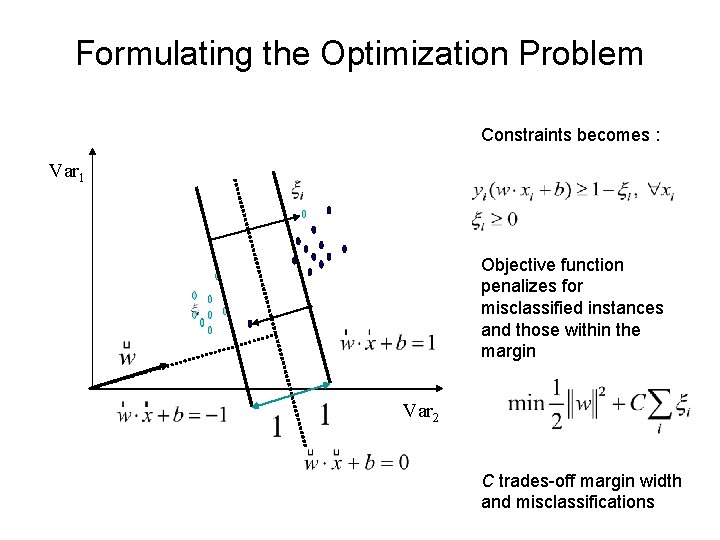
Formulating the Optimization Problem Constraints becomes : Var 1 Objective function penalizes for misclassified instances and those within the margin Var 2 C trades-off margin width and misclassifications
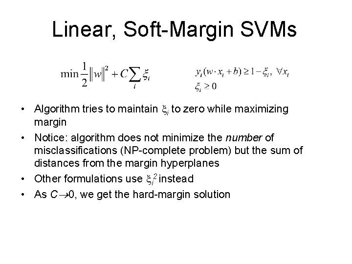
Linear, Soft-Margin SVMs • Algorithm tries to maintain i to zero while maximizing margin • Notice: algorithm does not minimize the number of misclassifications (NP-complete problem) but the sum of distances from the margin hyperplanes • Other formulations use i 2 instead • As C 0, we get the hard-margin solution
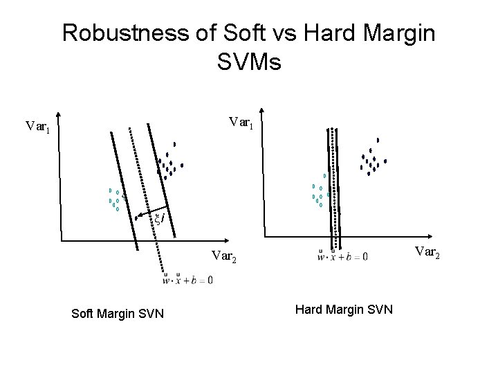
Robustness of Soft vs Hard Margin SVMs Var 1 i Var 2 Soft Margin SVN Hard Margin SVN
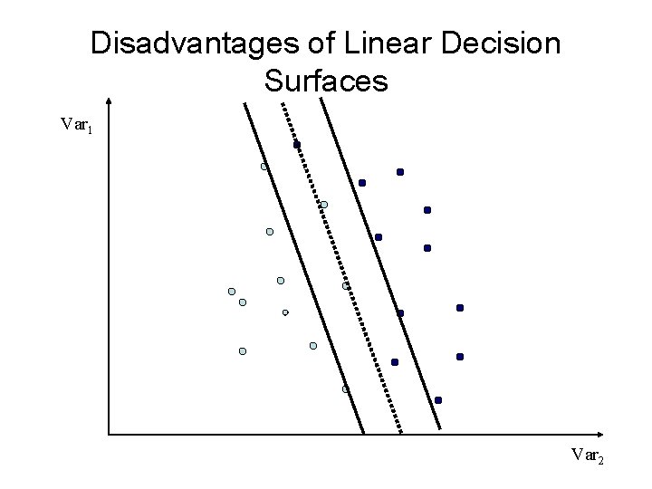
Disadvantages of Linear Decision Surfaces Var 1 Var 2
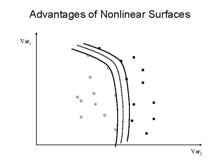
Advantages of Nonlinear Surfaces Var 1 Var 2
Methods I) Instance-based methods: 1) Nearest neighbor II) Probabilistic models: 1) Naïve Bayes 2) Logistic Regression III) Linear Models: 1) Perceptron 2) Support Vector Machine + kernel trick IV) Decision Models: 1) Decision Trees 2) Boosted Decision Trees 3) Random Forest
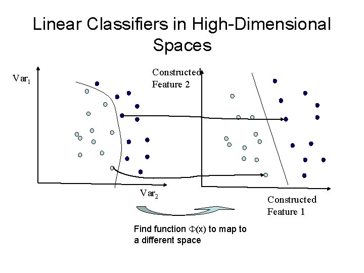
Linear Classifiers in High-Dimensional Spaces Var 1 Constructed Feature 2 Var 2 Find function (x) to map to a different space Constructed Feature 1
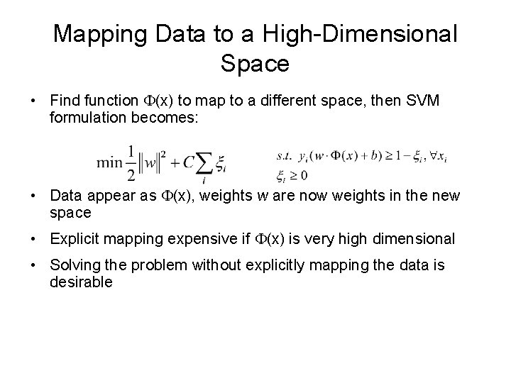
Mapping Data to a High-Dimensional Space • Find function (x) to map to a different space, then SVM formulation becomes: • Data appear as (x), weights w are now weights in the new space • Explicit mapping expensive if (x) is very high dimensional • Solving the problem without explicitly mapping the data is desirable
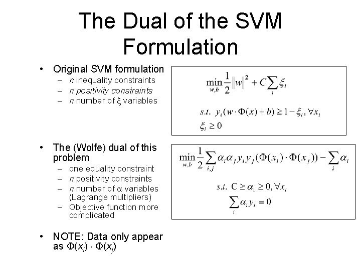
The Dual of the SVM Formulation • Original SVM formulation – n inequality constraints – n positivity constraints – n number of variables • The (Wolfe) dual of this problem – one equality constraint – n positivity constraints – n number of variables (Lagrange multipliers) – Objective function more complicated • NOTE: Data only appear as (xi) (xj)
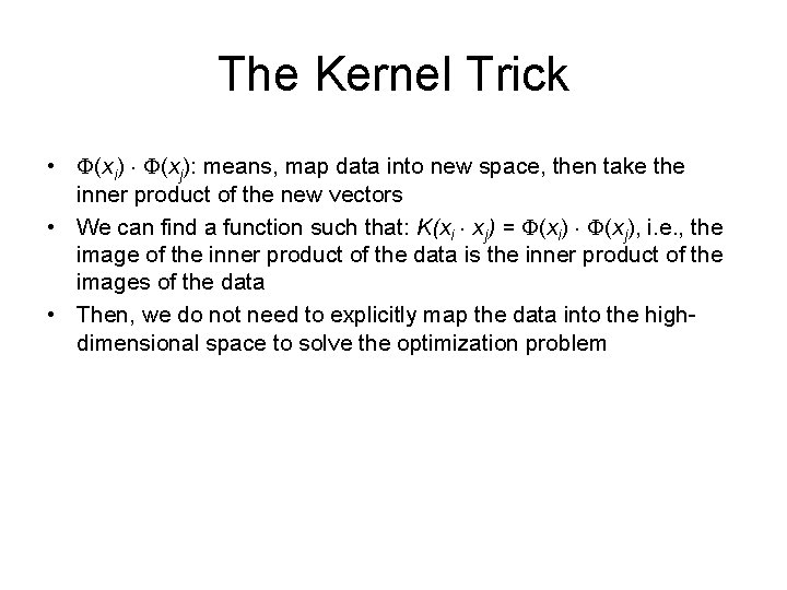
The Kernel Trick • (xi) (xj): means, map data into new space, then take the inner product of the new vectors • We can find a function such that: K(xi xj) = (xi) (xj), i. e. , the image of the inner product of the data is the inner product of the images of the data • Then, we do not need to explicitly map the data into the highdimensional space to solve the optimization problem
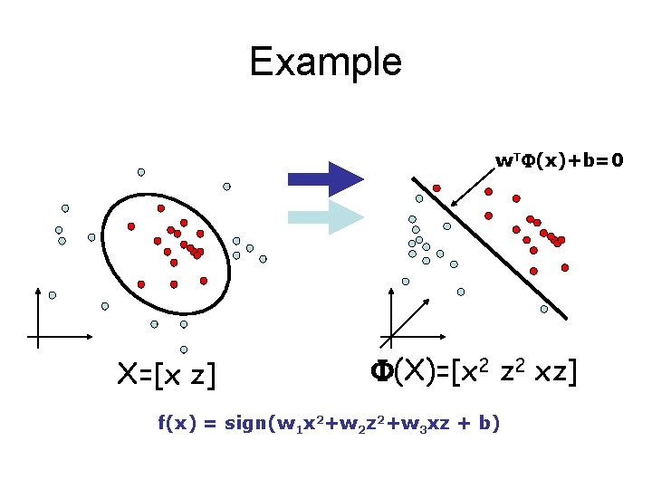
Example w. T (x)+b=0 X=[x z] (X)=[x 2 z 2 xz] f(x) = sign(w 1 x 2+w 2 z 2+w 3 xz + b)
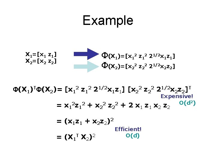
Example X 1=[x 1 z 1] X 2=[x 2 z 2] (X 1)=[x 12 z 12 21/2 x 1 z 1] (X 2)=[x 22 z 22 21/2 x 2 z 2] (X 1)T (X 2)= [x 12 z 12 21/2 x 1 z 1] [x 22 z 22 21/2 x 2 z 2]T Expensive! 2) O(d z = x 12 z 12 + x 22 z 22 + 2 x 1 z 1 x 2 = (x 1 z 1 + x 2 z 2)2 = (X 1 T X 2)2 Efficient! O(d) 2
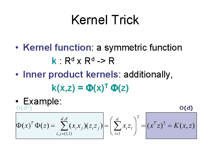
Kernel Trick • Kernel function: a symmetric function k : Rd x Rd -> R • Inner product kernels: additionally, k(x, z) = (x)T (z) • Example: O(d 2) O(d)
Kernel Trick • Implement an infinite-dimensional mapping implicitly • Only inner products explicitly needed for training and evaluation • Inner products computed efficiently, in finite dimensions • The underlying mathematical theory is that of reproducing kernel Hilbert space from functional analysis
Kernel Methods • If a linear algorithm can be expressed only in terms of inner products – it can be “kernelized” – find linear pattern in high-dimensional space – nonlinear relation in original space • Specific kernel function determines nonlinearity
Kernels • Some simple kernels – Linear kernel: k(x, z) = x. Tz equivalent to linear algorithm – Polynomial kernel: k(x, z) = (1+x. Tz)d polynomial decision rules – RBF kernel: k(x, z) = exp(-||x-z||2/2 ) highly nonlinear decisions
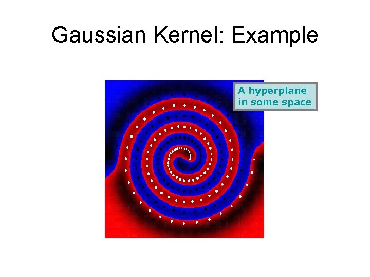
Gaussian Kernel: Example A hyperplane in some space
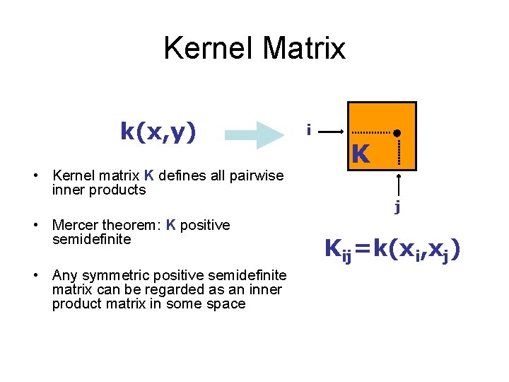
Kernel Matrix k(x, y) • Kernel matrix K defines all pairwise inner products • Mercer theorem: K positive semidefinite • Any symmetric positive semidefinite matrix can be regarded as an inner product matrix in some space i K j Kij=k(xi, xj)
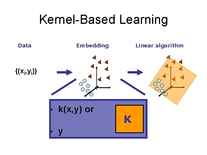
Kernel-Based Learning Data Embedding Linear algorithm {(xi, yi)} • k(x, y) or • y K
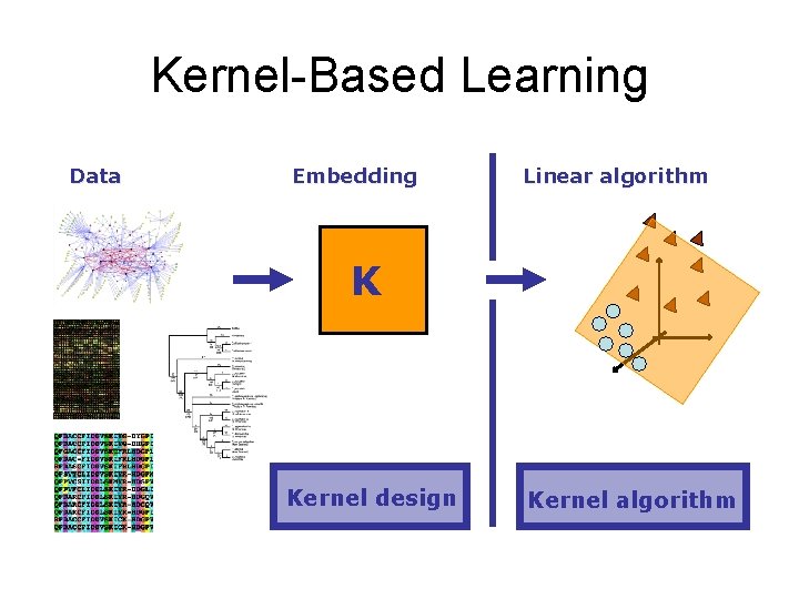
Kernel-Based Learning Data Embedding Linear algorithm K Kernel design Kernel algorithm
Kernel Design • Simple kernels on vector data • More advanced – string kernel – diffusion kernel – kernels over general structures (sets, trees, graphs. . . ) – kernels derived from graphical models – empirical kernel map
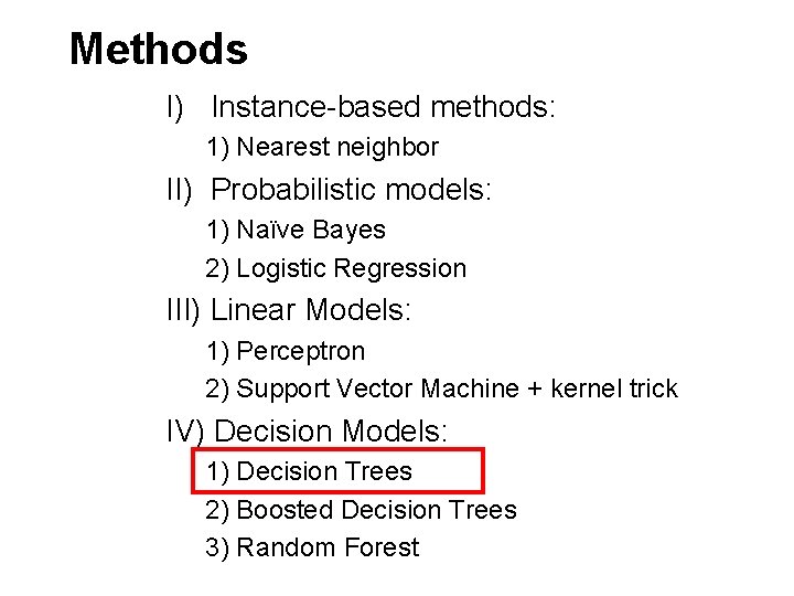
Methods I) Instance-based methods: 1) Nearest neighbor II) Probabilistic models: 1) Naïve Bayes 2) Logistic Regression III) Linear Models: 1) Perceptron 2) Support Vector Machine + kernel trick IV) Decision Models: 1) Decision Trees 2) Boosted Decision Trees 3) Random Forest
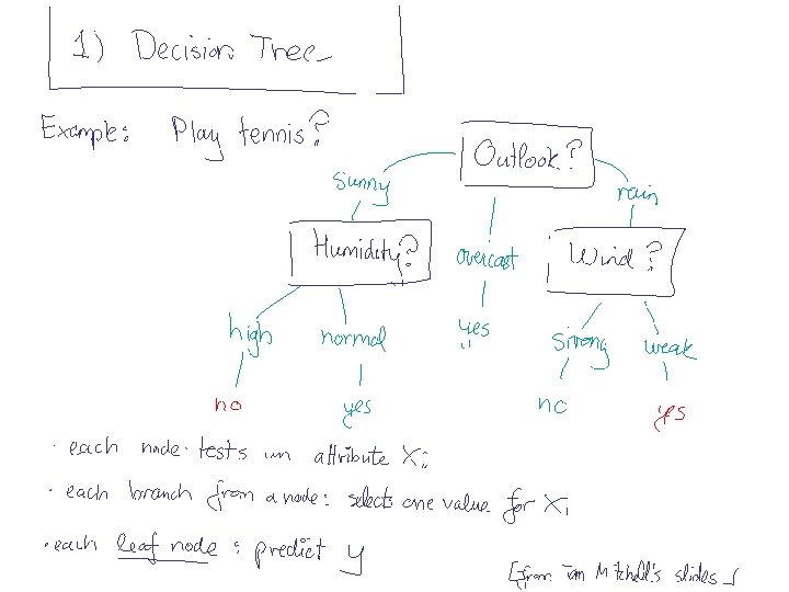
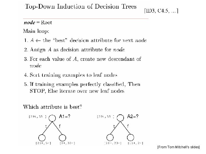
[From Tom Mitchell’s slides]
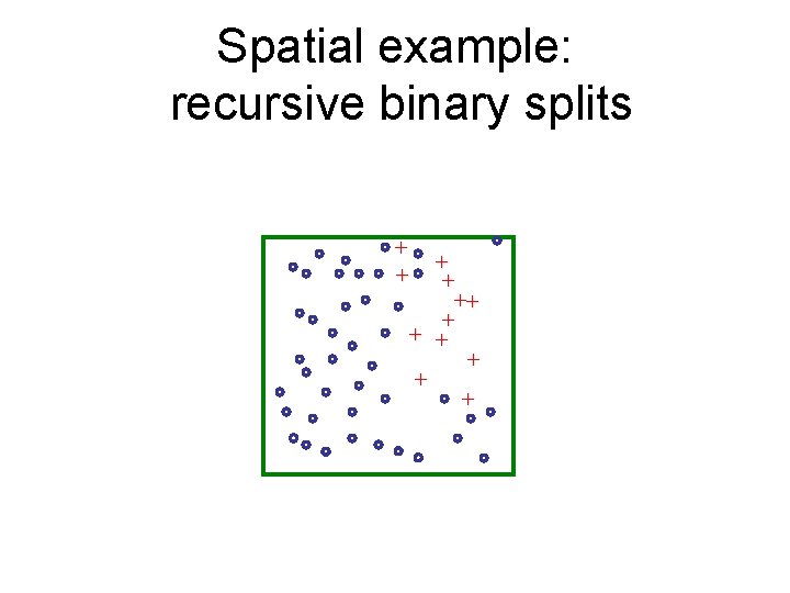
Spatial example: recursive binary splits + + ++ + + +
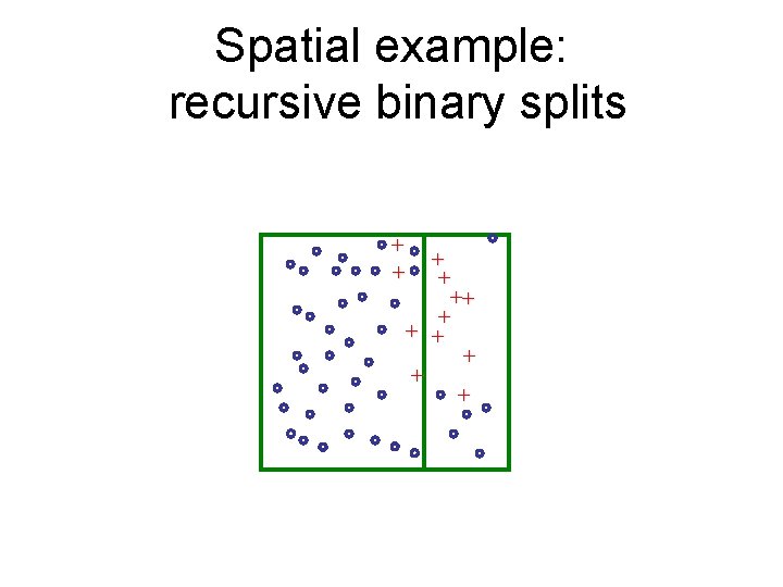
Spatial example: recursive binary splits + + ++ + + +
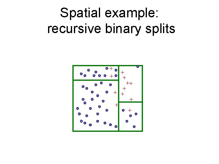
Spatial example: recursive binary splits + + ++ + + +
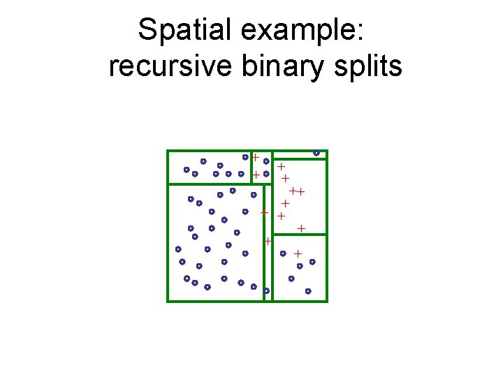
Spatial example: recursive binary splits + + ++ + + +
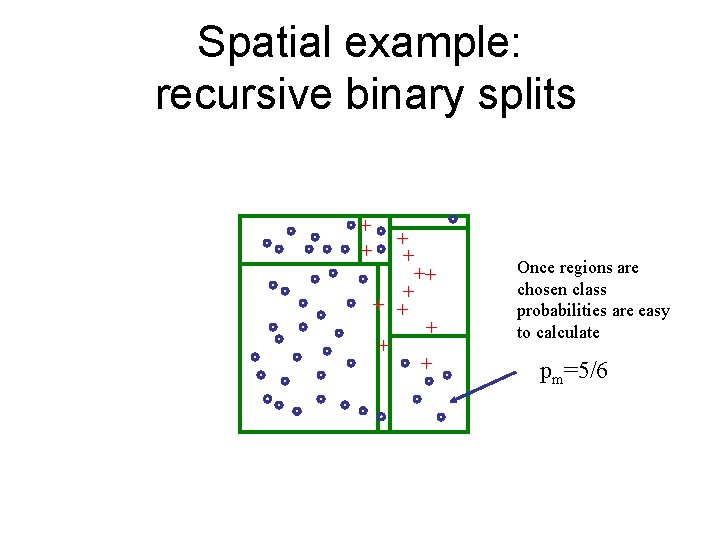
Spatial example: recursive binary splits + + ++ + + + Once regions are chosen class probabilities are easy to calculate pm=5/6
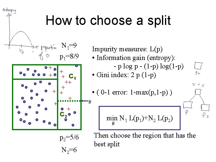
How to choose a split N 1=9 p 1=8/9 Impurity measures: L(p) • Information gain (entropy): - p log p - (1 -p) log(1 -p) • Gini index: 2 p (1 -p) + + C 1 ++ + + + C 2 p 2=5/6 N 2=6 • ( 0 -1 error: 1 -max(p, 1 -p) ) s min N 1 L(p 1)+N 2 L(p 2) s Then choose the region that has the best split
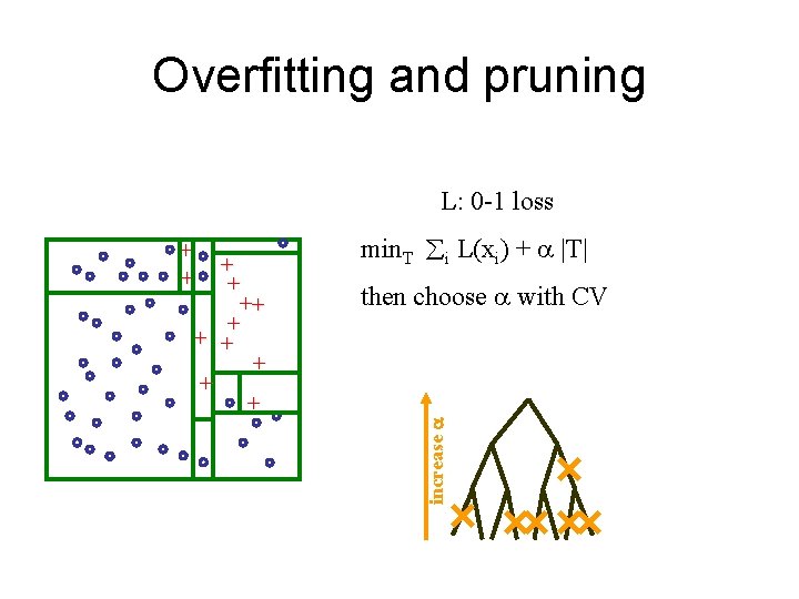
Overfitting and pruning L: 0 -1 loss + + + + + min. T åi L(xi) + |T| then choose with CV increase a + +
Methods I) Instance-based methods: 1) Nearest neighbor II) Probabilistic models: 1) Naïve Bayes 2) Logistic Regression III) Linear Models: 1) Perceptron 2) Support Vector Machine + kernel trick IV) Decision Models: 1) Decision Trees 2) Boosted Decision Trees 3) Random Forest
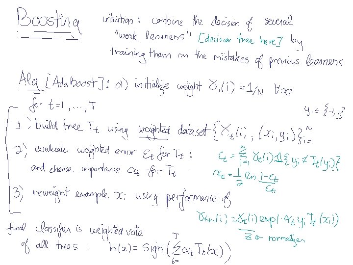
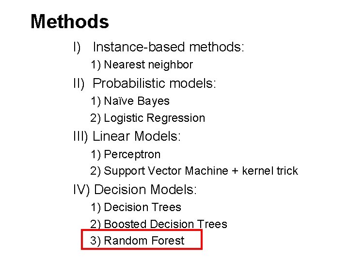
Methods I) Instance-based methods: 1) Nearest neighbor II) Probabilistic models: 1) Naïve Bayes 2) Logistic Regression III) Linear Models: 1) Perceptron 2) Support Vector Machine + kernel trick IV) Decision Models: 1) Decision Trees 2) Boosted Decision Trees 3) Random Forest
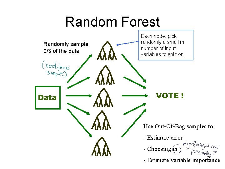
Random Forest Randomly sample 2/3 of the data Data Each node: pick randomly a small m number of input variables to split on VOTE ! Use Out-Of-Bag samples to: - Estimate error - Choosing m 79 - Estimate variable importance
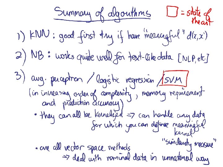
- Slides: 82