l 1106 Neural Nets Decision Trees Support Vector
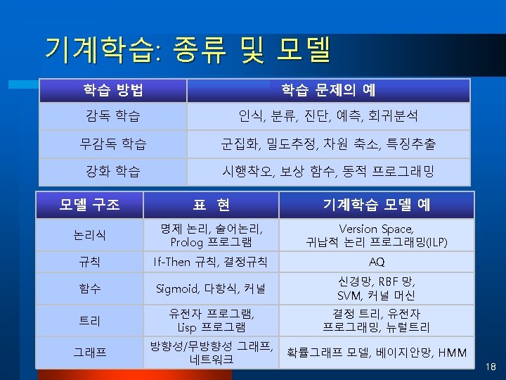
: 감독학습 ¨ Neural Nets ¨ Decision Trees ¨ Support Vector")


 Error Backpropagation Output Comparison Information Propagation Weights Input x 1 Input")
 NN learns to steer an autonomous vehicle. l")
 가정/사무실 도우미 로봇 l PR 2 Robot Cleans Up http: //www.")


![Example Applications l NETtalk [Sejnowski] ¨ Inputs: English text ¨ Output: Spoken phonemes l](https://slidetodoc.com/presentation_image_h/935879dad944b9c2d1eb5d065899d420/image-26.jpg "Example Applications l NETtalk [Sejnowski] ¨ Inputs: English text ¨ Output: Spoken phonemes l")
 NN learns to steer an autonomous vehicle. l 960")


 Perceptron: A neural net with a single neuron l Perceptron = a linear")
 Decision surface for a linearly separable set of")
")
 Error Linear unit (linear perceptron) l Note: output")


 Day Outlook Temperature Humidity Wind Play. Tennis D 1")
 (Outlook = Sunny")


 74")
 l Entropy of D SNU Center for Bioinformation Technology")
![Example : Play Tennis (2) l Attribute Wind ¨ D = [9+, 5 -]](https://slidetodoc.com/presentation_image_h/935879dad944b9c2d1eb5d065899d420/image-76.jpg "Example : Play Tennis (2) l Attribute Wind ¨ D = [9+, 5 -]")
![Example : Play Tennis (3) l Attribute Humidity ¨ Dhigh = [3+, 4 -]](https://slidetodoc.com/presentation_image_h/935879dad944b9c2d1eb5d065899d420/image-77.jpg "Example : Play Tennis (3) l Attribute Humidity ¨ Dhigh = [3+, 4 -]")
 l Best Attribute? ¨ Gain(D, Outlook) = 0. 246")
 l Entropy Dsunny Day Outlook Temperature Humidity Wind Play.")
![Example : Play Tennis (6) l Attribute Wind ¨ Dweak = [1+, 2 -]](https://slidetodoc.com/presentation_image_h/935879dad944b9c2d1eb5d065899d420/image-80.jpg "Example : Play Tennis (6) l Attribute Wind ¨ Dweak = [1+, 2 -]")
![Example : Play Tennis (7) l Attribute Humidity ¨ Dhigh = [0+, 3 -]](https://slidetodoc.com/presentation_image_h/935879dad944b9c2d1eb5d065899d420/image-81.jpg "Example : Play Tennis (7) l Attribute Humidity ¨ Dhigh = [0+, 3 -]")
 Best Attribute? l ¨ Gain(Dsunny, Humidity) = 0. 971")
 l Entropy Drain Day Outlook Temperature Humidity Wind Play.")
![Example : Play Tennis (10) l Attribute Wind ¨ Dweak = [3+, 0 -]](https://slidetodoc.com/presentation_image_h/935879dad944b9c2d1eb5d065899d420/image-84.jpg "Example : Play Tennis (10) l Attribute Wind ¨ Dweak = [3+, 0 -]")
![Example : Play Tennis (11) l Attribute Humidity ¨ Dhigh = [1+, 1 -]](https://slidetodoc.com/presentation_image_h/935879dad944b9c2d1eb5d065899d420/image-85.jpg "Example : Play Tennis (11) l Attribute Humidity ¨ Dhigh = [1+, 1 -]")
 l Best Attribute? ¨ Gain(Drain, Humidity) = 0. 020")

 88")


 ¨ Pima")
 Decision Tree (C) 2010, SNU")


 Memory-Based Learning (x, y=? ) Query Pattern (x 1,")
 xq Input (vector) … Hidden (vector)")
 l Training • For each training example <x, f(x)>, add")

 Hidden (scalar) Input (scalar) 106")


 l Rule extraction (after training) (Tresp")

 x 1 x 2 K(x, x")


- Slides: 140
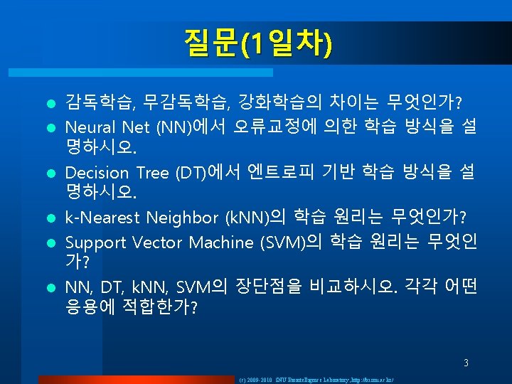
강의 개요 l 1일차(10/6): 감독학습 ¨ Neural Nets ¨ Decision Trees ¨ Support Vector Machines l 2일차(10/7): 무감독 학습 ¨ ¨ l Self-Organizing Maps Clustering Algorithms Reinforcement Learning Evolutionary Learning 3일차(10/8): 확률그래프모델 ¨ Bayesian Networks ¨ Markov Random Fields ¨ Particle Filters 2 (c) 2009 -2010 SNU Biointelligence Laboratory, http: //bi. snu. ac. kr/
Approaches to Artificial Intelligence Symbolic AI Rule-Based Systems Connectionist AI Neural Networks Evolutionary AI Genetic Algorithms Molecular AI: DNA Computing © 2007, SNU Biointelligence Lab, http: //bi. snu. ac. kr/ 4
Research Areas and Approaches Research Artificial Intelligence Application Paradigm Learning Algorithms Inference Mechanisms Knowledge Representation Intelligent System Architecture Intelligent Agents Information Retrieval Electronic Commerce Data Mining Bioinformatics Natural Language Proc. Expert Systems Rationalism (Logical) Empiricism (Statistical) Connectionism (Neural) Evolutionary (Genetic) Biological (Molecular) © 2007, SNU Biointelligence Lab, http: //bi. snu. ac. kr/ 5
Day 1 1. Concept of Machine Learning
Learning: Definition l Learning is the improvement of performance in some environment through the acquisition of knowledge resulting from experience in that environment. the improvement of behavior on some performance task through acquisition of knowledge based on partial task experience © 2010, SNU Biointelligence Lab, http: //bi. snu. ac. kr/ 7
Neural Network (MLP) Error Backpropagation Output Comparison Information Propagation Weights Input x 1 Input x 2 Output Input x 3 Input Layer Scaling Function Hidden Layer Activation Function Output Layer Activation Function © 2010, SNU Biointelligence Lab, http: //bi. snu. ac. kr/ 8
Application Example: Autonomous Land Vehicle (ALV) NN learns to steer an autonomous vehicle. l 960 input units, 4 hidden units, 30 output units l Driving at speeds up to 70 miles per hour l ALVINN System Image of a forward mounted camera Weight values for one of the hidden units © 2010, SNU Biointelligence Lab, http: //bi. snu. ac. kr/ 9
(참고: Willow Garage) 가정/사무실 도우미 로봇 l PR 2 Robot Cleans Up http: //www. youtube. com/watch? v=g Yqfa-Ytv. W 4&feature=related l PR 2 Robot Plays Pool http: //www. youtube. com/watch? v= mg. HUNfq. Ih. Ac&feature=related PR 2 Robot of Willow Garage 12 © 2010, SNU Biointelligence Lab, http: //bi. snu. ac. kr/
Machine Learning: Three Tasks l Supervised Learning l Unsupervised Learning l Reinforcement Learning ¨ Estimate an unknown mapping from known input and target output pairs ¨ Learn fw from training set D={(x, y)} s. t. ¨ Classification: y is discrete ¨ Regression: y is continuous ¨ ¨ Only input values are provided Learn fw from D={(x)} s. t. Compression Clustering ¨ ¨ Not target, but rewards (critiques) are provided Learn a heuristic function hw from D={(x, a, c)} s. t. Action selection Policy learning © 2007, SNU Biointelligence Lab, http: //bi. snu. ac. kr/ 16
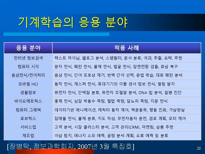
기계학습 기술: 대표적인 알고리즘 l Symbolic Learning l ¨ Bayesian Networks ¨ Helmholtz Machines ¨ Version Space Learning ¨ Case-Based Learning l l ¨ Markov Random Fields ¨ Hypernetworks Neural Learning ¨ ¨ Multilayer Perceptrons Self-Organizing Maps Support Vector Machines Kernel Machines Evolutionary Learning ¨ ¨ ¨ Evolution Strategies Evolutionary Programming Genetic Algorithms Genetic Programming Molecular Programming Probabilistic Learning ¨ Latent Variable Models ¨ Generative Topographic Mapping l Other Methods ¨ ¨ ¨ Decision Trees Reinforcement Learning Boosting Algorithms Mixture of Experts Independent Component Analysis © 2007, SNU Biointelligence Lab, http: //bi. snu. ac. kr/ 19
Day 1 2. Neural Network Learning
From Biological Neuron to Artificial Neuron Dendrite Cell Body Axon
From Biology to Artificial Neural Nets
Properties of Artificial Neural Networks l A network of artificial neurons l Characteristics t t t <Multilayer Perceptron Network> Nonlinear I/O mapping Adaptivity Generalization ability Fault-tolerance (graceful degradation) Biological analogy
Problems Appropriate for Neural Networks l Many training examples available l Outputs can be discrete or continuous-valued or their vectors. l May contain noise in training examples l Tolerant to long training time l Fast execution time l Not necessary to explain the prediction results
Example Applications l NETtalk [Sejnowski] ¨ Inputs: English text ¨ Output: Spoken phonemes l Phoneme recognition [Waibel] ¨ Inputs: wave form features ¨ Outputs: b, c, d, … l Robot control [Pomerleau] ¨ Inputs: perceived features ¨ Outputs: steering control
Application: Autonomous Land Vehicle (ALV) NN learns to steer an autonomous vehicle. l 960 input units, 4 hidden units, 30 output units l Driving at speeds up to 70 miles per hour l ALVINN System Image of a forward mounted camera Weight values for one of the hidden units
Application: Data Recorrection by a Hopfield Network original target data Recorrected data after 10 iterations corrupted input data Recorrected data after 20 iterations Fully recorrected data after 35 iterations
Perceptron and Gradient Descent Algorithm
(Simple) Perceptron: A neural net with a single neuron l Perceptron = a linear threshold unit (LTU) ¨ Note: Linear perceptron = linear unit (see below) Input: a vector of real values l Output: 1 or -1 (binary) l Activation function: threshold function l
Linearly Separable vs. Linearly Nonseparable (a) Decision surface for a linearly separable set of examples (correctly classified by a straight line) (b) A set of training examples that is not linearly separable.
Perceptron Training Rule Note: output value o is +1 or -1 (not a real) l Perceptron rule: a learning rule for a threshold unit. l Conditions for convergence l ¨ Training examples are linearly separable. ¨ Learning rate is sufficiently small.
Delta Rule: Least Mean Square (LMS) Error Linear unit (linear perceptron) l Note: output value o is a real value (not binary) l Delta rule: learning rule for an unthresholded perceptron (i. e. linear unit). l ¨ Delta rule is a gradient-descent rule.
Gradient Descent Method
Delta Rule for Error Minimization
Perceptron Learning Algorithm
Multilayer Perceptron
Multilayer Perceptrons x 1 y 1 … x 2 … … ym xn Input layer Hidden layer Output layer • x: input vector • y: output vector • Supervised learning • Gradient search • Noise immunity • Learning algorithm: Backpropagation © 2007, SNU Biointelligence Lab, http: //bi. snu. ac. kr/ 38
Multilayer Networks and its Decision Boundaries * * Decision regions of a multilayer feedforward network. The network was trained to recognize 1 of 10 vowel sounds occurring in the context “h_d” The network input consists of two parameter, F 1 and F 2, obtained from a spectral analysis of the sound. The 10 network outputs correspond to the 10 possible vowel sounds.
Differentiable Threshold Unit l Sigmoid function: nonlinear, differentiable
Error Function for BP l l E defined as a sum of the squared errors over all the output units k for all the training examples d. Error surface can have multiple local minima ¨ Guarantee toward some local minimum ¨ No guarantee to the global minimum
Backpropagation Learning Algorithm for MLP
Adding Momentum l Original weight update rule for BP: l Adding momentum ¨ Help to escape a small local minima in the error surface. ¨ Speed up the convergence.
Derivation of the BP Rule l Notations ¨ xij : the ith input to unit j ¨ wij : the weight associated with the ith input to unit j ¨ netj : the weighted sum of inputs for unit j ¨ oj : the output computed by unit j ¨ tj : the target output for unit j ¨ : the sigmoid function ¨ outputs : the set of units in the final layer of the network ¨ Downstream(j) : the set of units whose immediate inputs include the output of unit j
Derivation of the BP Rule l Error measure: l Gradient descent: l Chain rule:
Case 1: Rule for Output Unit Weights l Step 1: l Step 2: l Step 3: l All together:
Case 2: Rule for Hidden Unit Weights l Step 1: l Thus:
BP for MLP: revisited
Hidden Layer Representations BP has an ability to discover useful intermediate representations at the hidden unit layers inside the networks which capture properties of the input spaces that are most relevant to learning the target function. l When more layers of units are used in the network, more complex features can be invented. l But the representations of the hidden layers are very hard to understand for humans. l
Hidden Layer Representation for Identity Function
Hidden Layer Representation for Identity Function * The evolving sum of squared errors for each of the eight output units as the number of training iterations (epochs) increase
Hidden Layer Representation for Identity Function * The evolving hidden layer representation for the input string “ 01000000”
Hidden Layer Representation for Identity Function * The evolving weights for one of the three hidden units
Generalization and Overfitting l Continuing training until the training error falls below some predetermined threshold is a poor strategy since BP is susceptible to overfitting. ¨ Need to measure the generalization accuracy over a validation set (distinct from the training set). l Two different types of overffiting ¨ Generalization error first decreases, then increases, even the training error continues to decrease. ¨ Generalization error decreases, then increases, then decreases again, while the training error continues to decreases.
Two Kinds of Overfitting Phenomena
Techniques for Overcoming the Overfitting Problem l Weight decay ¨ Decrease each weight by some small factor during each iteration. ¨ This is equivalent to modifying the definition of E to include a penalty term corresponding to the total magnitude of the network weights. ¨ The motivation for the approach is to keep weight values small, to bias learning against complex decision surfaces l k-fold cross-validation ¨ Cross validation is performed k different times, each time using a different partitioning of the data into training and validation sets ¨ The result are averaged after k times cross validation.
Designing an Artificial Neural Network for Face Recognition Application
ANN for Face Recognition 960 x 3 x 4 network is trained on gray-level images of faces to predict whether a person is looking to their left, right, ahead, or up.
Problem Definition l Possible learning tasks ¨ Classifying camera images of faces of people in various poses. ¨ Direction, Identity, Gender, . . . l Data: ¨ 624 grayscale images for 20 different people ¨ 32 images person, varying < person’s expression (happy, sad, angry, neutral) < direction (left, right, straight ahead, up) < with and without sunglasses ¨ resolution of images: 120 x 128, each pixel with a grayscale intensity between 0 (black) and 255 (white) l Task: Learning the direction in which the person is facing.
Factors for ANN Design in the Face Recognition Task Input encoding Output encoding Network graph structure Other learning algorithm parameters
Input Coding for Face Recognition l Possible Solutions ¨ Extract key features using preprocessing ¨ Coarse-resolution l Features extraction ¨ edges, regions of uniform intensity, other local image features ¨ Defect: High preprocessing cost, variable number of features l Coarse-resolution ¨ Encode the image as a fixed set of 30 x 32 pixel intensity values, with one network input per pixel. ¨ The 30 x 32 pixel image is a coarse resolution summary of the original 120 x 128 pixel image ¨ Coarse-resolution reduces the number of inputs and weights to a much more manageable size, thereby reducing computational demands.
Output Coding for Face Recognition l Possible coding schemes ¨ Using one output unit with multiple threshold values ¨ Using multiple output units with single threshold value. l One unit scheme ¨ Assign 0. 2, 0. 4, 0. 6, 0. 8 to encode four-way classification. l Multiple units scheme (1 -of-n output encoding) ¨ Use four distinct output units ¨ Each unit represents one of the four possible face directions, with highest-valued output taken as the network prediction
Output Coding for Face Recognition l Advantages of 1 -of-n output encoding scheme ¨ It provides more degrees of freedom to the network for representing the target function. ¨ The difference between the highest-valued output and the second-highest can be used as a measure of the confidence in the network prediction. l Target value for the output units in 1 -of-n encoding scheme ¨ < 1, 0, 0, 0 > v. s. < 0. 9, 0. 1, 0. 1 > ¨ < 1, 0, 0, 0 >: will force the weights to grow without bound. ¨ < 0. 9, 0. 1, 0. 1 >: the network will have finite weights.
Network Structure for Face Recognition One hidden layer v. s. more hidden layers l How many hidden nodes is used? l ¨ Using 3 hidden units: < test accuracy for the face data = 90% < Training time = 5 min on Sun Sprac 5 ¨ Using 30 hidden units: < test accuracy for the face data = 91. 5% < Training time = 1 hour on Sun Sparc 5
Other Parameters for Face Recognition Learning rate = 0. 3 l Momentum = 0. 3 l Weight initialization: small random values near 0 l Number of iterations: Cross validation l ¨ After every 50 iterations, the performance of the network was evaluated over the validation set. ¨ The final selected network is the one with the highest accuracy over the validation set
Day 1 3. Decision Tree Learning
Decision Trees Nodes: attributes l Edges: values l Terminal nodes: class labels l quicktime no yes YES unix yes no computer no yes NO space ` NO no clinton no NO l yes Learning Algorithm: C 4. 5 YES yes YES © 2007, SNU Biointelligence Lab, http: //bi. snu. ac. kr/ 67
Main Idea Classification by Partitioning Example Space l Goal : Approximating discrete-valued target functions l Appropriate Problems l ¨ ¨ Examples are represented by attribute-value pairs. The target function has discrete output value. Disjunctive description may be required. The training data may contain missing attribute values. SNU Center for Bioinformation Technology (CBIT) 68
q Example Problem (Play Tennis) Day Outlook Temperature Humidity Wind Play. Tennis D 1 D 2 D 3 D 4 D 5 D 6 D 7 D 8 D 9 D 10 D 11 D 12 D 13 D 14 Sunny Overcast Rain Overcast Sunny Rain Sunny Overcast Rain Hot Hot Mild Cool Mild Hot Mild High Normal Normal High Weak Strong Weak Weak Strong Weak Strong No No Yes Yes Yes No
Example Space No Yes (Outlook = Sunny & Humidity = High) (Outlook = Sunny & Humidity = Normal) Yes (Outlook = Overcast) Yes No (Outlook = Rain & Wind = Weak) (Outlook = Rain & Wind = Strong) SNU Center for Bioinformation Technology (CBIT) 70
Decision Tree Representation Outlook Sunny Humidity High NO Overcast Rain Wind YES Normal YES NO SNU Center for Bioinformation Technology (CBIT) YES 71
Basic Decision Tree Learning l Which Attribute is Best? ¨ Select the attribute that is most useful for classifying examples. ¨ Quantitative Measure Information Gain < For Attribute A, relative to a collection of data D < < Expected Reduction of Entropy SNU Center for Bioinformation Technology (CBIT) 72
Entropy Impurity of an Arbitrary Collection of Examples l Minimum number of bits of information needed to encode the classification of an arbitrary member of D 1. 0 Entropy(S) l 0. 0 SNU Center for Bioinformation Technology (CBIT) 1. 0 73
Constructing Decision Tree SNU Center for Bioinformation Technology (CBIT) 74
Example : Play Tennis (1) l Entropy of D SNU Center for Bioinformation Technology (CBIT) 75
Example : Play Tennis (2) l Attribute Wind ¨ D = [9+, 5 -] ¨ Dweak = [6+, 2 -] ¨ Dstrong=[3+, 3 -] [9+, 5 -] : E = 0. 940 Wind Weak [6+, 2 -] : E = 0. 811 SNU Center for Bioinformation Technology (CBIT) Strong [3+, 3 -] : E = 1. 0 76
Example : Play Tennis (3) l Attribute Humidity ¨ Dhigh = [3+, 4 -] ¨ Dnormal=[6+, 1 -] [9+, 5 -] : E = 0. 940 Humidity High [3+, 4 -] : E = 0. 985 SNU Center for Bioinformation Technology (CBIT) Normal [6+, 1 -] : E = 0. 592 77
Example : Play Tennis (4) l Best Attribute? ¨ Gain(D, Outlook) = 0. 246 ¨ Gain(D, Humidity) = 0. 151 ¨ Gain(D, Wind) = 0. 048 ¨ Gain(D, Temperature) = 0. 029 [9+, 5 -] : E = 0. 940 Outlook Sunny Overcast [2+, 3 -] : (D 1, D 2, D 8, D 9, D 11) [4+, 0 -] : (D 3, D 7, D 12, D 13) YES Rain [3+, 2 -] : (D 4, D 5, D 6, D 10, D 14) SNU Center for Bioinformation Technology (CBIT) 78
Example : Play Tennis (5) l Entropy Dsunny Day Outlook Temperature Humidity Wind Play. Tennis D 1 D 2 D 8 D 9 D 11 Sunny Sunny Hot Mild Cool Mild High Normal Weak Strong No No No Yes SNU Center for Bioinformation Technology (CBIT) 79
Example : Play Tennis (6) l Attribute Wind ¨ Dweak = [1+, 2 -] ¨ Dstrong=[1+, 1 -] [2+, 3 -] : E = 0. 971 Wind Weak [1+, 2 -] : E = 0. 918 SNU Center for Bioinformation Technology (CBIT) Strong [1+, 1 -] : E = 1. 0 80
Example : Play Tennis (7) l Attribute Humidity ¨ Dhigh = [0+, 3 -] ¨ Dnormal=[2+, 0 -] [2+, 3 -] : E = 0. 971 Humidity High [0+, 3 -] : E = 0. 00 SNU Center for Bioinformation Technology (CBIT) Normal [2+, 0 -] : E = 0. 00 81
Example : Play Tennis (8) Best Attribute? l ¨ Gain(Dsunny, Humidity) = 0. 971 ¨ Gain(Dsunny, Wind) = 0. 020 ¨ Gain(Dsunny, Temperature) = 0. 571 [9+, 5 -] : E = 0. 940 Outlook Sunny Humidity High NO Overcast YES Normal Rain [3+, 2 -] : (D 4, D 5, D 6, D 10, D 14) YES SNU Center for Bioinformation Technology (CBIT) 82
Example : Play Tennis (9) l Entropy Drain Day Outlook Temperature Humidity Wind Play. Tennis D 4 D 5 D 6 D 10 D 14 Rain Rain Mild Cool Mild High Normal High Weak Strong Yes No SNU Center for Bioinformation Technology (CBIT) 83
Example : Play Tennis (10) l Attribute Wind ¨ Dweak = [3+, 0 -] ¨ Dstrong=[0+, 2 -] [3+, 2 -] : E = 0. 971 Wind Weak [3+, 0 -] : E = 0. 00 SNU Center for Bioinformation Technology (CBIT) Strong [0+, 2 -] : E = 0. 00 84
Example : Play Tennis (11) l Attribute Humidity ¨ Dhigh = [1+, 1 -] ¨ Dnormal=[2+, 1 -] [2+, 3 -] : E = 0. 971 Humidity High [1+, 1 -] : E = 1. 00 SNU Center for Bioinformation Technology (CBIT) Normal [2+, 1 -] : E = 0. 918 85
Example : Play Tennis (12) l Best Attribute? ¨ Gain(Drain, Humidity) = 0. 020 ¨ Gain(Drain, Wind) = 0. 971 ¨ Gain(Drain, Temperature) = 0. 020 Sunn y Humidity High NO Outlook Overcas t YES Rain Wind Normal YES SNU Center for Bioinformation Technology (CBIT) NO YES 86
Avoiding Overfitting Data l Definition ¨ Given a hypothesis space H, a hypothesis h H is said to overfit the data if there exists some alternative hypothesis h’ H, such that h has smaller error than h’ over the training examples, but h’ has a smaller error than h over entire distribution of instances. l Occam’s Razor ¨ Prefer the simplest hypothesis that fits the data. SNU Center for Bioinformation Technology (CBIT) 87
Avoiding Overfitting Data SNU Center for Bioinformation Technology (CBIT) 88
Solutions to Overfitting 1. Partition examples into training, test, and validation set. 2. Use all data for training, but apply a statistical test to estimate whether expanding (or pruning) a particular node is likely to produce an improvement beyond the training set. 3. Use an explicit measure of the complexity for encoding the training examples and the decision tree, halting growth of the tree when this encoding is minimized. SNU Center for Bioinformation Technology (CBIT) 89
Summary Decision trees provide a practical method for concept learning and discrete-valued functions. l ID 3 searches a complete hypothesis space. l Overfitting is an important issue in decision tree learning. l SNU Center for Bioinformation Technology (CBIT) 90
Day 1 4 -5. 실습
Plan for ML Exercise l Day 1: Classification ¨ Program: Weka ¨ Agenda: classification by Neural Network(NN) and Decision Tree (DT) l Day 2: Clustering ¨ Program: Genesis ¨ Agenda: k-means /hierarchical clustering, SOM l Day 3: Bayesian Network ¨ Program: Ge. NIe ¨ Agenda: designing / learning / inference in Bayesian networks (C) 2010, SNU Biointelligence Lab, http: //bi. snu. ac. kr/
Day 1 Classification – The Tool for Practice l Weka 3: Data Mining Software in Java ¨ Collection of machine learning algorithms for data mining tasks ¨ What you can do with Weka are < data pre-processing, feature selection, classification, regression, clustering, association rules, and visualization ¨ Weka is an open source software issued under the GNU General Public License ¨ How to get? http: //www. cs. waikato. ac. nz/ml/weka/ or just type ‘Weka’ in google. (C) 2010, SNU Biointelligence Lab, http: //bi. snu. ac. kr/
Classification Using Weka - Problems l Pima Indians Diabetes (2 -class problem) ¨ Pima Indians have the highest prevalence of diabetes in the world ¨ We will build classification models that diagnoses if the patient shows signs of diabetes l Handwritten Digit Recognition (10 -class problem) ¨ The MNIST database of handwritten digits contains digits written by office workers and students ¨ We will build a recognition model based on classifiers with the reduced set of MNIST (C) 2010, SNU Biointelligence Lab, http: //bi. snu. ac. kr/
Classification Using Weka - Algorithms Neural Network (Multilayer Perceptron) Decision Tree (C) 2010, SNU Biointelligence Lab, http: //bi. snu. ac. kr/
Classification Using Weka click • load a file that contains the training data by clicking ‘Open file’ button • ‘ARFF’ or ‘CSV’ formats are readible • Click ‘Multilayer. Perceptron’ • Set parameters for MLP • Set parameters for Test • Click ‘Start’ for learning (C) 2010, SNU Biointelligence Lab, http: //bi. snu. ac. kr/ • Click ‘Classify’ tab • Click ‘Choose’ button • Select ‘weka – function - Multilayer. Perceptron
Classification Using Weka Options for testing the trained model Result output: various measures appear (C) 2010, SNU Biointelligence Lab, http: //bi. snu. ac. kr/
Day 1 6. k-Nearest Neighbor
Different Learning Methods l Eager learning ¨ Explicit description of target function on the whole training set l Instance-based learning ¨ Learning = storing all training instances ¨ Classification = assigning a target function to a new instance ¨ Referred to as “lazy” learning l Kinds of instance-based learning ¨ K-nearest neighbor algorithm ¨ Locally weighted regression ¨ Case-based reasoning
Local vs. Distributed Representation Lazy Learning? Eager Learning 100
K-Nearest Neighbor l Features ¨ All instances correspond to points in an n-dimensional Euclidean space ¨ Classification is delayed till a new instance arrives ¨ Classification done by comparing feature vectors of the different points ¨ Target function may be discrete or real-valued
k-Nearest Neighbor Classifier (k. NN) Memory-Based Learning (x, y=? ) Query Pattern (x 1, y 1=1) (x 2, y 2=1) (x 3, y 3=0) (x 4, y 4=0) (x 5, y 5=1) (x 6, y 6=0). . . (x. N, y. N=1) Learning Set D k=5 1 1 0 0 Three 1’s vs. Two 0’s y=1 1 Match Set © 2010, SNU Biointelligence Lab, http: //bi. snu. ac. kr/ 102
k. NN as a Neural Network (xi, yi) xq Input (vector) … Hidden (vector) yq Output (vector) 103
k-Nearest Neighbor (k. NN) l Training • For each training example <x, f(x)>, add the example to the learning set D Classification • Given a query instance xq, denote the k l instances from D that are nearest to xq • Return xq + + + where (a, b)=1 if a=b, and (a, b)=0 otherwise. l Memory-based or case-based learning © 2010, SNU Biointelligence Lab, http: //bi. snu. ac. kr/ 104
Generalizing k. NN l Divide the input space into local regions and learn simple (constant/linear) models in each patch Unsupervised: Competitive, online clustering l Supervised: Radial-basis func, mixture of experts l 105
Radial-Basis Function Network Locally-tuned units Output (scalar) Hidden (scalar) Input (scalar) 106
Training RBF Hybrid learning: ¨ First layer centers and spreads: Unsupervised k-means ¨ Second layer weights: Supervised gradient-descent l Fully supervised l (Broomhead and Lowe, 1988; Moody and Darken, 1989) l 107
Regression 108
Classification 109
Rules and Exceptions 110 Default rule
Rule-Based Knowledge Incorporation of prior knowledge (before training) l Rule extraction (after training) (Tresp et al. , 1997) l Fuzzy membership functions and fuzzy rules l 111
Day 1 7. Support Vector Machines
Support Vector Machines Bias b K(x, x 1) x 1 x 2 K(x, x 2) Input layer y Output neuron … … xn Type of SVM K(x, xm) Inner product kernel K(x, xi) Polynomial learning machine Radial-basis function network Two-layer perceptron Hidden layer of m inner-product kernels © 2010, SNU Biointelligence Lab, http: //bi. snu. ac. kr/ 113
Support Vector Machines The line that maximizes the minimum margin is a good bet. ¨ The model class of “hyper-planes with a margin of m” has a low VC dimension if m is big. l This maximum-margin separator is determined by a subset of the datapoints. ¨ Datapoints in this subset are called “support vectors”. ¨ It will be useful computationally if only a small fraction of the datapoints are support vectors, because we use the support vectors to decide which side of the separator a test case is on. l The support vectors are indicated by the circles around them.
Training a linear SVM l To find the maximum margin separator, we have to solve the following optimization problem: l This is tricky but it’s a convex problem. There is only one optimum and we can find it without fiddling with learning rates or weight decay or early stopping. ¨ Don’t worry about the optimization problem. It has been solved. Its called quadratic programming. ¨ It takes time proportional to N^2 which is really bad for very big datasets < so for big datasets we end up doing approximate optimization!
Testing a linear SVM l The separator is defined as the set of points for which:
Introducing slack variables l Slack variables are constrained to be non-negative. When they are greater than zero they allow us to cheat by putting the plane closer to the datapoint than the margin. So we need to minimize the amount of cheating. This means we have to pick a value for lamba (this sounds familiar!)
A picture of the best plane with a slack variable
How to make a plane curved Fitting hyperplanes as separators is mathematically easy. ¨ The mathematics is linear. l By replacing the raw input variables with a much larger set of features we get a nice property: ¨ A planar separator in the highdimensional space of feature vectors is a curved separator in the low dimensional space of the raw input variables. l A planar separator in a 20 -D feature space projected back to the original 2 -D space
A potential problem and a magic solution l l If we map the input vectors into a very high-dimensional feature space, surely the task of finding the maximum-margin separator becomes computationally intractable? ¨ The mathematics is all linear, which is good, but the vectors have a huge number of components. ¨ So taking the scalar product of two vectors is very expensive. The way to keep things tractable is to use “the kernel trick” l The kernel trick makes your brain hurt when you first learn about it, but its actually very simple.
The kernel trick l For many mappings from a low-D space to a high-D space, there is a simple operation on two vectors in the low-D space that can be used to compute the scalar product of their two images in the high-D space. Letting the kernel do the work doing the scalar product in the obvious way Low-D High-D
Kernel Examples 1. Gaussian kernel 2. Polynomial kernel
The classification rule l The final classification rule is quite simple: The set of support vectors All the cleverness goes into selecting the support vectors that maximize the margin and computing the weight to use on each support vector. l We also need to choose a good kernel function and we may need to choose a lambda for dealing with non-separable cases. l
Some commonly used kernels Polynomial: Gaussian radial basis function Parameters that the user must choose Neural net: For the neural network kernel, there is one “hidden unit” per support vector, so the process of fitting the maximum margin hyperplane decides how many hidden units to use. Also, it may violate Mercer’s condition.
Support Vector Machines are Perceptrons! SVM’s use each training case, x, to define a feature K(x, . ) where K is chosen by the user. ¨ So the user designs the features. l Then they do “feature selection” by picking the support vectors, and they learn how to weight the features by solving a big optimization problem. l So an SVM is just a very clever way to train a standard perceptron. ¨ All of the things that a perceptron cannot do cannot be done by SVM’s (but it’s a long time since 1969 so people have forgotten this). l
Supplement: SVM as a Kernel Machine
Kernel Methods Approach l The kernel methods approach is to stick with linear functions but work in a high dimensional feature space: The expectation is that the feature space has a much higher dimension than the input space. l
Form of the Functions l So kernel methods use linear functions in a feature space: l For regression this could be the function l For classification require thresholding
Controlling generalisation l The critical method of controlling generalisation is to force a large margin on the training data:
Support Vector Machines l SVM optimization Addresses generalization issue but not the computational cost of dealing with large vectors l
Complexity problem l Let’s apply the quadratic example to a 20 x 30 image of 600 pixels – gives approximately 180000 dimensions! l Would be computationally infeasible to work in this space
Dual Representation l Suppose weight vector is a linear combination of the training examples: l can evaluate inner product with new example
Learning the dual variables Since any component orthogonal to the space spanned by the training data has no effect, general result that weight vectors have dual representation: the representer theorem. l Hence, can reformulate algorithms to learn dual variables rather than weight vector directly l
Dual Form of SVM l The dual form of the SVM can also be derived by taking the dual optimisation problem! This gives: l Note that threshold must be determined from border examples
Using Kernels Critical observation is that again only inner products are used l Suppose that we now have a shortcut method of computing: l l Then we do not need to explicitly compute the feature vectors either in training or testing
Kernel example l As an example consider the mapping l Here we have a shortcut:
Efficiency Hence, in the pixel example rather than work with 180000 dimensional vectors, we compute a 600 dimensional inner product and then square the result! l Can even work in infinite dimensional spaces, eg using the Gaussian kernel: l
Constraints on the kernel l There is a restriction on the function: l This restriction for any training set is enough to guarantee function is a kernel
What Have We Achieved? Replaced problem of neural network architecture by kernel definition l ¨ Arguably more natural to define but restriction is a bit unnatural ¨ Not a silver bullet as fit with data is key ¨ Can be applied to non- vectorial (or high dim) data Gained more flexible regularization/ generalization control l Gained convex optimization problem l ¨ i. e. NO local minima! l However, choosing the right kernel remains as a design issue.