CS 188 Artificial Intelligence Neural Nets and Decision


 z 1")
 z 1 f 2(x)")
 x 2")

![Common Activation Functions [source: MIT 6. S 191 introtodeeplearning. com]](https://slidetodoc.com/presentation_image/0e7c5e3fa3356be1f59bb6b3fe297dec/image-8.jpg "Common Activation Functions [source: MIT 6. S 191 introtodeeplearning. com]")

. A two-layer neural network with a")


 x 1 x 2 … x 3 … …")


![What’s still missing? – correlation neq causation [Ribeiro et al. ]](https://slidetodoc.com/presentation_image/0e7c5e3fa3356be1f59bb6b3fe297dec/image-33.jpg "What’s still missing? – correlation neq causation [Ribeiro et al. ]")
![What’s still missing? – covariate shift [Carroll et al. ]](https://slidetodoc.com/presentation_image/0e7c5e3fa3356be1f59bb6b3fe297dec/image-34.jpg "What’s still missing? – covariate shift [Carroll et al. ]")
![What’s still missing? – covariate shift [Carroll et al. ]](https://slidetodoc.com/presentation_image/0e7c5e3fa3356be1f59bb6b3fe297dec/image-35.jpg "What’s still missing? – covariate shift [Carroll et al. ]")

 =")


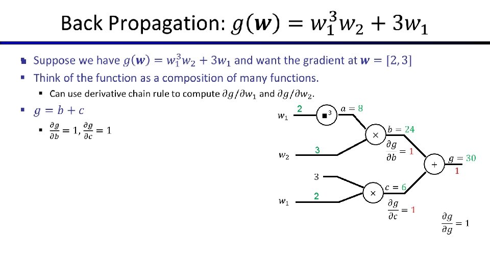
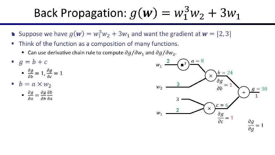
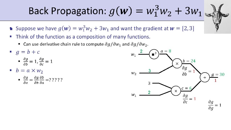
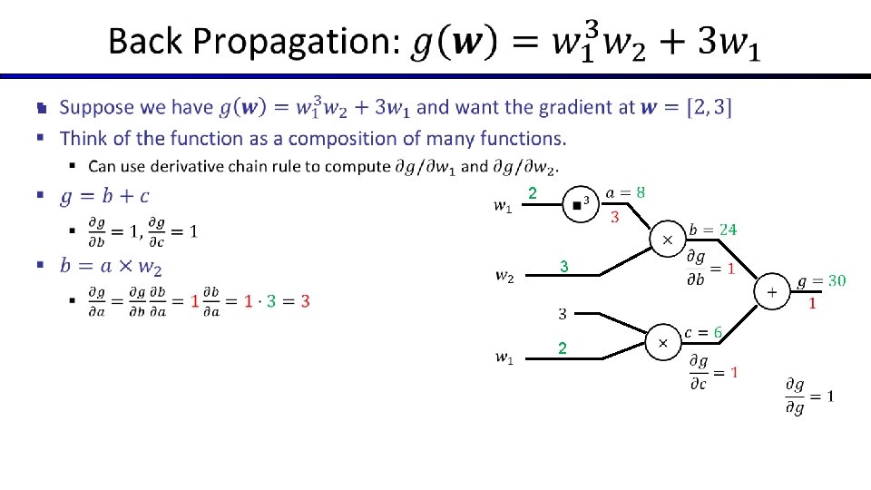
 § Simplest form: learn a function from examples § A target")
: § Consistency vs. simplicity § Ockham’s")

- Slides: 65
CS 188: Artificial Intelligence Neural Nets and Decision Trees Instructor: Nathan Lambert --- University of California, Berkeley [These slides were created by Dan Klein, Pieter Abbeel, Sergey Levine. All CS 188 materials are at http: //ai. berkeley. edu. ]
Neural Net Demo! https: //playground. tensorflow. org/
Neural Networks
Multi-class Logistic Regression § = special case of neural network f 1(x) z 1 f 2(x) f 3(x) … f. K(x) z 2 z 3 s o f t m a x
Deep Neural Network = Also learn the features! f 1(x) z 1 f 2(x) f 3(x) … f. K(x) z 2 z 3 s o f t m a x
Deep Neural Network = Also learn the features! x 1 f 1(x) x 2 f 2(x) … x 3 … x. L f 3(x) … … s o f t m a x f. K(x) g = nonlinear activation function
Deep Neural Network = Also learn the features! x 1 x 2 … x 3 … … … s o f t m a x x. L g = nonlinear activation function
Common Activation Functions [source: MIT 6. S 191 introtodeeplearning. com]
Deep Neural Network: Also Learn the Features! § Training the deep neural network is just like logistic regression: just w tends to be a much, much larger vector just run gradient ascent + stop when log likelihood of hold-out data starts to decrease
Neural Networks Properties § Theorem (Universal Function Approximators). A two-layer neural network with a sufficient number of neurons can approximate any continuous function to any desired accuracy. § Practical considerations § Can be seen as learning the features § Large number of neurons § Danger for overfitting § (hence early stopping!)
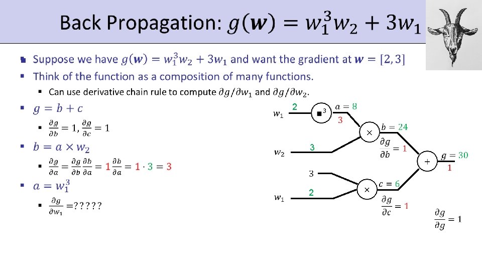
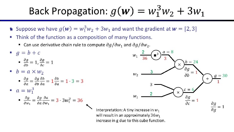
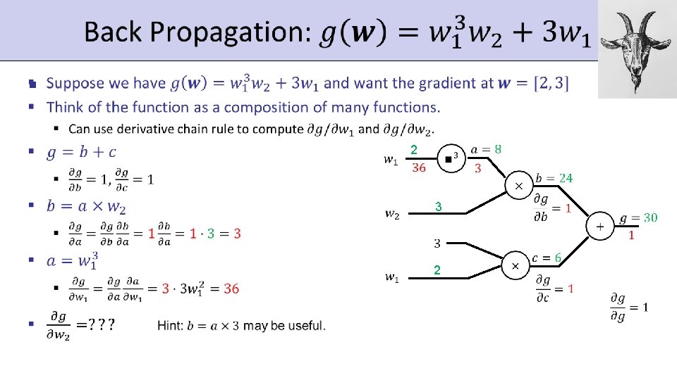
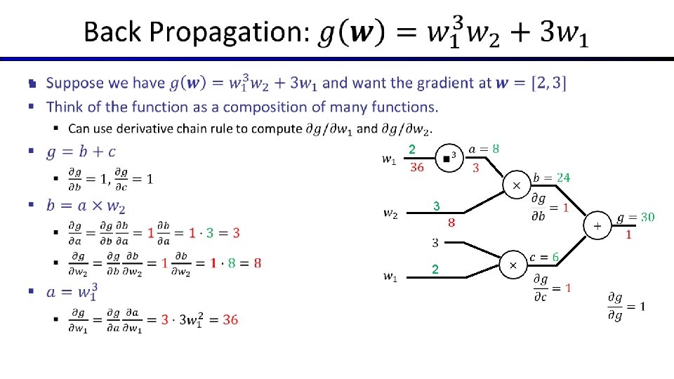
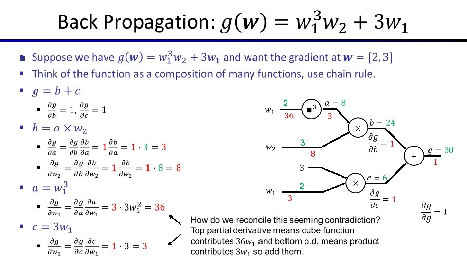
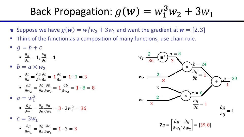
How about computing all the derivatives? § Derivatives tables: [source: http: //hyperphysics. phy-astr. gsu. edu/hbase/Math/derfunc. html
How about computing all the derivatives? n But neural net f is never one of those? n No problem: CHAIN RULE: If Then Derivatives can be computed by following well-defined procedures
Automatic Differentiation § Automatic differentiation software e. g. Theano, Tensor. Flow, Py. Torch, Chainer Only need to program the function g(x, y, w) Can automatically compute all derivatives w. r. t. all entries in w This is typically done by caching info during forward computation pass of f, and then doing a backward pass = “backpropagation” § Autodiff / Backpropagation can often be done at computational cost comparable to the forward pass § § § Need to know this exists § How this is done? -- outside of scope of CS 188
Training a Network (setting weights) x 1 x 2 … x 3 … … … s o f t m a x x. L g = nonlinear activation function
Training a Network Key words: • • Forward Backwards Gradient Backprop … … s o f t m a x g = nonlinear activation function
Gradient Descent §
Summary of Key Ideas § Optimize probability of label given input § Continuous optimization § Gradient ascent: § Compute steepest uphill direction = gradient (= just vector of partial derivatives) § Take step in the gradient direction § Repeat (until held-out data accuracy starts to drop = “early stopping”) § Deep neural nets § Last layer = still logistic regression § Now also many more layers before this last layer § = computing the features § the features are learned rather than hand-designed § Universal function approximation theorem § If neural net is large enough § Then neural net can represent any continuous mapping from input to output with arbitrary accuracy § But remember: need to avoid overfitting / memorizing the training data early stopping! § Automatic differentiation gives the derivatives efficiently (how? = outside of scope of 188)
Computer Vision
Manual Feature Design
Features and Generalization Image Ho. G
Performance Alex. Net graph credit Matt Zeiler, Clarifai
Speech Recognition graph credit Matt Zeiler, Clarifai
What’s still missing? – correlation neq causation [Ribeiro et al. ]
What’s still missing? – covariate shift [Carroll et al. ]
What’s still missing? – covariate shift [Carroll et al. ]
Decision Trees
Reminder: Features § Features, aka attributes § Sometimes: TYPE=French § Sometimes: f. TYPE=French(x) = 1
Decision Trees § Compact representation of a function: § Truth table § Conditional probability table § Regression values § True function § Realizable: in H
Expressiveness of DTs § Can express any function of the features § However, we hope for compact trees
Comparison: Perceptrons § What is the expressiveness of a perceptron over these features? § For a perceptron, a feature’s contribution is either positive or negative § If you want one feature’s effect to depend on another, you have to add a new conjunction feature § E. g. adding “PATRONS=full WAIT = 60” allows a perceptron to model the interaction between the two atomic features § DTs automatically conjoin features / attributes § Features can have different effects in different branches of the tree! § Difference between modeling relative evidence weighting (NB) and complex evidence interaction (DTs) § Though if the interactions are too complex, may not find the DT greedily
Decision Tree Learning § Aim: find a small tree consistent with the training examples § Idea: (recursively) choose “most significant” attribute as root of (sub)tree
Choosing an Attribute § Idea: a good attribute splits the examples into subsets that are (ideally) “all positive” or “all negative” § So: we need a measure of how “good” a split is, even if the results aren’t perfectly separated out
Entropy and Information § Information answers questions § The more uncertain about the answer initially, the more information in the answer § Scale: bits § § Answer to Boolean question with prior <1/2, 1/2>? Answer to 4 -way question with prior <1/4, 1/4>? Answer to 4 -way question with prior <0, 0, 0, 1>? Answer to 3 -way question with prior <1/2, 1/4>? § A probability p is typical of: § A uniform distribution of size 1/p § A code of length log 1/p
Entropy § General answer: if prior is <p 1, …, pn>: § Information is the expected code length 1 bit § Also called the entropy of the distribution 0 bits § More uniform = higher entropy § More values = higher entropy § More peaked = lower entropy 0. 5 bit
Information Gain § Back to decision trees! § For each split, compare entropy before and after § Difference is the information gain § Problem: there’s more than one distribution after split! § Solution: use expected entropy, weighted by the number of examples
Next Step: Recurse § Now we need to keep growing the tree! § Two branches are done (why? ) § What to do under “full”? § See what examples are there…
Example: Learned Tree § Decision tree learned from these 12 examples: § Substantially simpler than “true” tree § A more complex hypothesis isn't justified by data § Also: it’s reasonable, but wrong
40 Examples Example: Miles Per Gallon
Find the First Split § Look at information gain for each attribute § Note that each attribute is correlated with the target! § What do we split on?
Result: Decision Stump
Second Level
Final Tree
Reminder: Overfitting § Overfitting: § When you stop modeling the patterns in the training data (which generalize) § And start modeling the noise (which doesn’t) § We had this before: § Naïve Bayes: needed to smooth § Perceptron: early stopping
MPG Training Error The test set error is much worse than the training set error… …why?
Significance of a Split § Starting with: § Three cars with 4 cylinders, from Asia, with medium HP § 2 bad MPG § 1 good MPG § What do we expect from a three-way split? § Maybe each example in its own subset? § Maybe just what we saw in the last slide? § Probably shouldn’t split if the counts are so small they could be due to chance § A chi-squared test can tell us how likely it is that deviations from a perfect split are due to chance* § Each split will have a significance value, p. CHANCE
Keeping it General § Pruning: § Build the full decision tree § Begin at the bottom of the tree § Delete splits in which p. CHANCE > Max. PCHANCE § Continue working upward until there are no more prunable nodes y = a XOR b
Pruning example § With Max. PCHANCE = 0. 1: Note the improved test set accuracy compared with the unpruned tree
Regularization § Max. PCHANCE is a regularization parameter § Generally, set it using held-out data (as usual) Accuracy Training Held-out / Test Decreasing Small Trees High Bias Max. PCHANCE Increasing Large Trees High Variance
Forward Pointer: Random Forests § Ensemble method of learning trees § Very effective, used in industry and more § Related to Boosting
A few important points about learning § Data: labeled instances, e. g. emails marked spam/ham § Training set § Held out set § Test set § Features: attribute-value pairs which characterize each x § Experimentation cycle § § § Learn parameters (e. g. model probabilities) on training set (Tune hyperparameters on held-out set) Compute accuracy of test set Very important: never “peek” at the test set! Evaluation § Accuracy: fraction of instances predicted correctly § Training Data Held-Out Data Overfitting and generalization § Want a classifier which does well on test data § Overfitting: fitting the training data very closely, but not generalizing well § Underfitting: fits the training set poorly Test Data
A few important points about learning § What should we learn where? § Learn parameters from training data § Tune hyperparameters on different data § Why? § For each value of the hyperparameters, train and test on the held-out data § Choose the best value and do a final test on the test data § What are examples of hyperparameters?
Inductive Learning
Inductive Learning (Science) § Simplest form: learn a function from examples § A target function: g § Examples: input-output pairs (x, g(x)) § E. g. x is an email and g(x) is spam / ham § E. g. x is a house and g(x) is its selling price § Problem: § Given a hypothesis space H § Given a training set of examples xi § Find a hypothesis h(x) such that h ~ g § Includes: § Classification (outputs = class labels) § Regression (outputs = real numbers) § How do perceptron and naïve Bayes fit in? (H, h, g, etc. )
Inductive Learning § Curve fitting (regression, function approximation): § Consistency vs. simplicity § Ockham’s razor
Consistency vs. Simplicity § Fundamental tradeoff: bias vs. variance § Usually algorithms prefer consistency by default (why? ) § Several ways to operationalize “simplicity” § Reduce the hypothesis space § Assume more: e. g. independence assumptions, as in naïve Bayes § Have fewer, better features / attributes: feature selection § Other structural limitations (decision lists vs trees) § Regularization § Smoothing: cautious use of small counts § Many other generalization parameters (pruning cutoffs today) § Hypothesis space stays big, but harder to get to the outskirts