GMS 573 RME slide set 03 The Risks

GMS 573 (RME): slide set 03 The Risks of Clinical Treatment • Suppose you diagnose a medical condition and decide upon a treatment • Will your treatment be effective and restore your patient to good health? • Or, will your treatment be ineffective, perhaps even harmful? • It depends on many factors, not the least important of which is your choice of treatment • Now we’ll consider the risks of treatment choice, and we’ll begin with the story about Bendectin (a. k. a. , Debendox in England Diclectin in Canada), an anti-nausea drug

GMS 573 (RME): slide set 03 The Risks of Clinical Treatment • A landmark U. S. Supreme Court case in 1993 involved Bendectin • Bendectin was developed originally by Merrell Dow, Inc. , in the 1960’s for relief of so-called “morning sickness” during early pregnancy (NVP: nausea and vomiting of pregnancy) • Bendectin was designed to be a safe alternative to the infamous Thalidomide medication of the 1950’s • 1970 -1980: prescription Bendectin was used by roughly 30% of all pregnant women in the U. S. • In 1984, Merrell Dow voluntarily withdrew Bendectin from the commercial market

GMS 573 (RME): slide set 03 Was Bendectin Safe to Use? • Minor limb-reduction birth defects occur naturally in low rates (roughly 20 per 1, 000 live births = 0. 2% of all births) • The problem was to decide whether the rate of minor birth defects in women who had used the drug was greater than the rate in women who had not used the drug • The government solution was to use retrospective studies • By the early 1970’s the federal government had examined 30 articles published in peer-review journals involving roughly 130, 000 women, some who had taken Bendectin, and others who had not • The birth records were examined and the women were surveyed on their medical histories

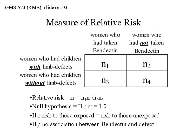
GMS 573 (RME): slide set 03 Measure of Relative Risk • Relative risk = rr = n 1 n 4/n 2 n 3 • Null hypothesis = H 0: rr = 1. 0 • H 0: risk to those exposed = risk to those unexposed • H 0: no association between Bendectin and defect

GMS 573 (RME): slide set 03 Standard of Proof • It is impossible to prove that a drug is safe with 100% certainty • But it is possible to show that it is NOT safe using the standard of a < 0. 05, i. e. , if H 0: rr = 1. 0 is rejected • The federal government found that peer-reviewed retrospective studies using a < 0. 05 as the standard had consistently failed to reject the null hypothesis that the use of Bendectin was not associated with the occurrence of limb reduction birth defects • The studies had not proven that Bendectin could not cause the birth defects…they merely showed that the rate of birth defects among Bendectin users was not statistically greater than the rate among non-users • Still, in 1984, Merrell Dow withdrew Bendectin from market

GMS 573 (RME): slide set 03 The Daubert Case • In 1988 a woman sued Merrell Dow, claiming that she had used Bendectin during her pregnancy before it had been withdrawn from the market, and that she had subsequently given birth to a child with a limb-reduction birth defect • Her claim was that the company had negligently marketed an unsafe drug, and by the way, she claimed that the government had negligently approved an unsafe drug • Plaintiff’s attorneys used a novel argument: they claimed that peer-reviewed medical research using the a < 0. 05 standard in publication should not be interpreted as meeting any legal standard of evidence • They also argued that scientific evidence based on “a < 0. 05” reasoning should be inadmissible in any product liability case

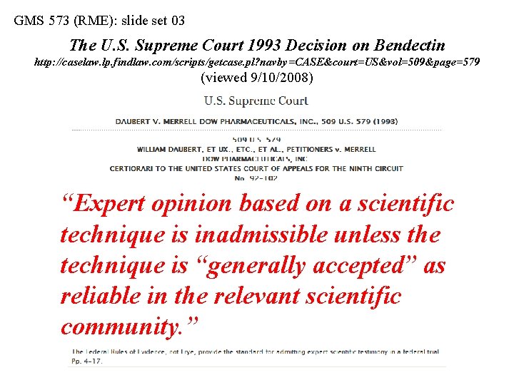
GMS 573 (RME): slide set 03 The Supreme Court Decision in 1993 • Daubert v. Merrel Dow Pharmaceuticals, Inc. , 509 U. S. 579 (1993). William Daubert, et ux. , et al. , Petitioners v. Merrell Dow Pharmaceuticals, Inc. Certiorari to the United States Court of Appeals for the Ninth Circuit, No. 92 -102, argued March 30, 1993, decided June 28, 1993 • The Supreme Court found that the so-called “Frye standard” could be applied in the Bendectin case • The Frye standard was a legal precedent established in 1923 regarding the admissibility of scientific evidence in legal proceedings (see: Frye v. United States (293 F. 1013 [DC Cir 1923]). • Frye was strictly about admissibility of polygraph evidence introduced in court, but it applied broadly to scientific evidence

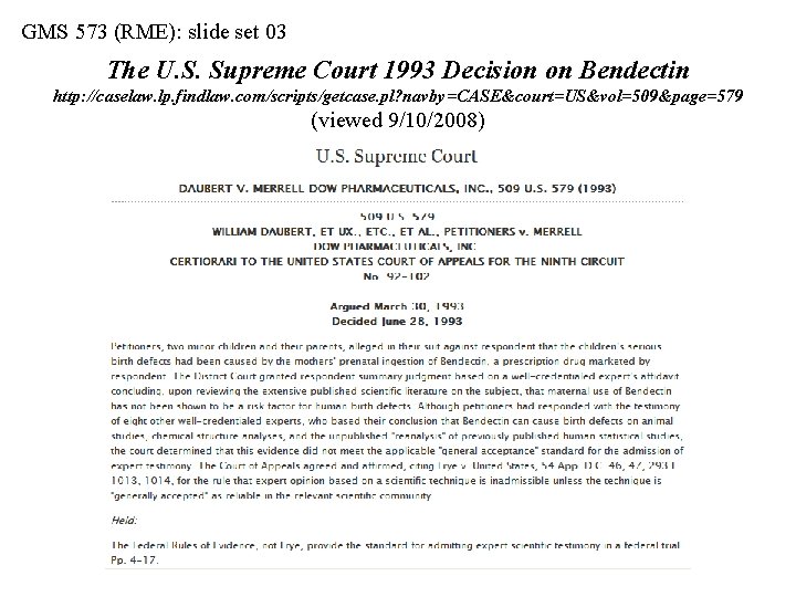
GMS 573 (RME): slide set 03 The U. S. Supreme Court 1993 Decision on Bendectin http: //caselaw. lp. findlaw. com/scripts/getcase. pl? navby=CASE&court=US&vol=509&page=579 (viewed 9/10/2008)

GMS 573 (RME): slide set 03 The U. S. Supreme Court 1993 Decision on Bendectin http: //caselaw. lp. findlaw. com/scripts/getcase. pl? navby=CASE&court=US&vol=509&page=579 (viewed 9/10/2008) “Expert opinion based on a scientific technique is inadmissible unless the technique is “generally accepted” as reliable in the relevant scientific community. ”

GMS 573 (RME): slide set 03 The Meaning of Daubert v. Merrell Dow • The decision recognized a < 0. 05 reasoning as valid in expert opinion concerning scientific evidence presented in court • The phrase “generally accepted technique” referred specifically to a < 0. 05 reasoning • That is, the court recognized the general acceptance among scientists in this approach to hypothesis testing • Consequences for our statistical decision… • H 0: Bendectin and birth defects are not associated • HA: Bendectin and birth defects are associated

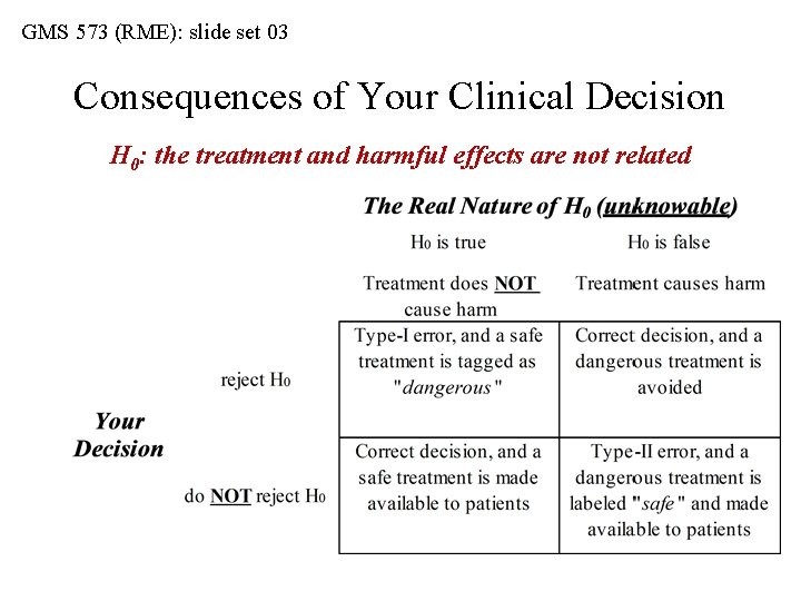
GMS 573 (RME): slide set 03 Consequences of Your Clinical Decision H 0: the treatment and harmful effects are not related

GMS 573 (RME): slide set 03 Other One-Sample Hypotheses • So far, we've looked at single variables such as body weight BMI, serum cholesterol, pulse, etc. • Often in biomedical research, the investigator is interested in the relationship between variables within a single sample • Suppose we could sample randomly in a population and draw out the "ith" individual, and measure more than one value • Thus, we have a one-sample design involving more than one variable • The best example of this is in the concept of statistical correlation and/or regression

GMS 573 (RME): slide set 03 Correlation vs. Regression • Does variation of one variable correlate in any way with variation in the other? • Correlation refers to statistical methods which allow you to infer about the relationship between these variables, i. e. , the degree to which two variables vary together • Can the value of one variable be used to predict the value of the other? • Regression refers to the statistical methods which allow you to infer whether variation in one variable (Y, the dependent variable) is caused by variation in the other variable (X, the independent variable)

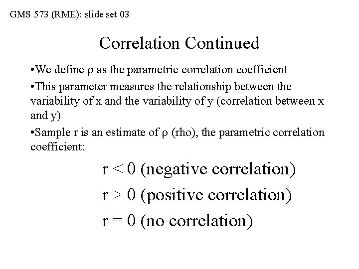
GMS 573 (RME): slide set 03 Correlation Continued • We define as the parametric correlation coefficient • This parameter measures the relationship between the variability of x and the variability of y (correlation between x and y) • Sample r is an estimate of (rho), the parametric correlation coefficient: r < 0 (negative correlation) r > 0 (positive correlation) r = 0 (no correlation)

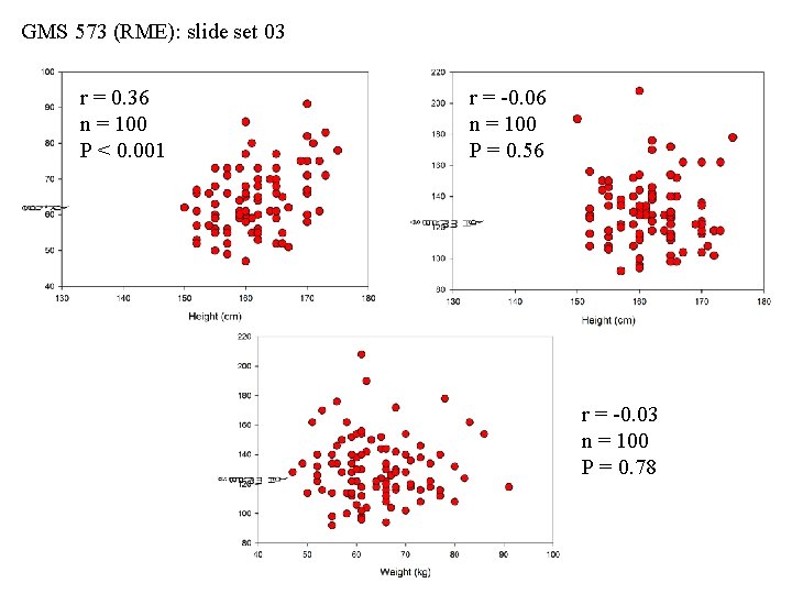
GMS 573 (RME): slide set 03 Correlation Continued • The sample is used to test the null hypothesis: "there is no correlation between the variables, " or: H 0: = 0 • There is actually a modified t-test you can use on your sample data and the sample r • In fact Excel today can calculate the sample r-values for you very quickly • Let’s use some data from the Honolulu Heart Study • Use height (cm), weight (kg), and sys BP (mm Hg)

GMS 573 (RME): slide set 03 r = 0. 36 n = 100 P < 0. 001 r = -0. 06 n = 100 P = 0. 56 r = -0. 03 n = 100 P = 0. 78

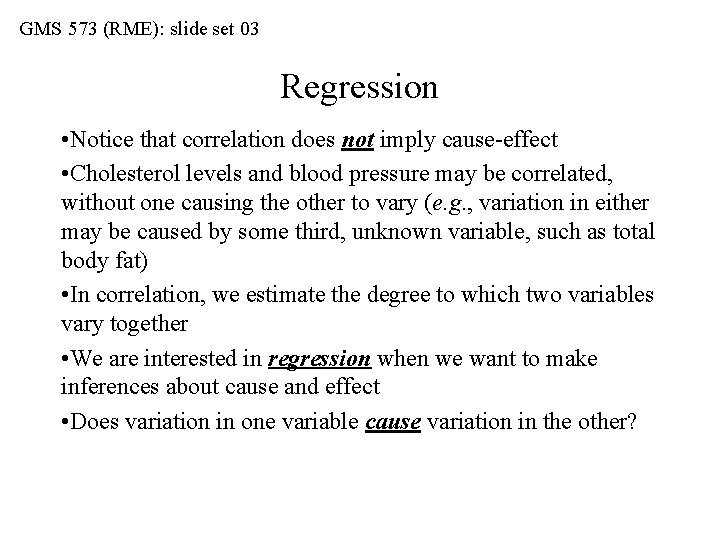
GMS 573 (RME): slide set 03 Regression • Notice that correlation does not imply cause-effect • Cholesterol levels and blood pressure may be correlated, without one causing the other to vary (e. g. , variation in either may be caused by some third, unknown variable, such as total body fat) • In correlation, we estimate the degree to which two variables vary together • We are interested in regression when we want to make inferences about cause and effect • Does variation in one variable cause variation in the other?

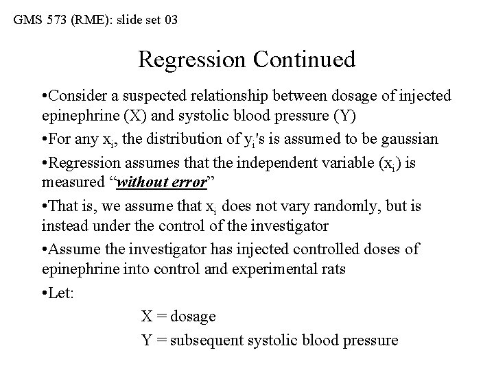
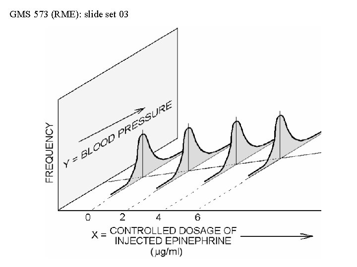
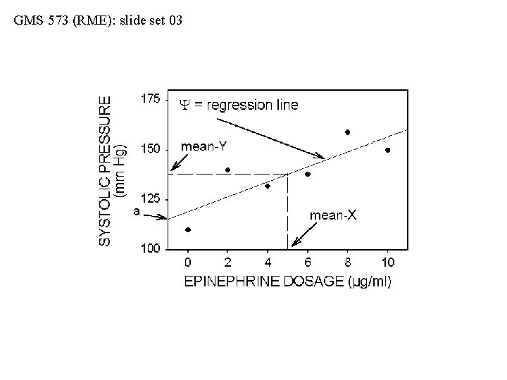
GMS 573 (RME): slide set 03 Regression Continued • Consider a suspected relationship between dosage of injected epinephrine (X) and systolic blood pressure (Y) • For any xi, the distribution of yi's is assumed to be gaussian • Regression assumes that the independent variable (xi) is measured “without error” • That is, we assume that xi does not vary randomly, but is instead under the control of the investigator • Assume the investigator has injected controlled doses of epinephrine into control and experimental rats • Let: X = dosage Y = subsequent systolic blood pressure

GMS 573 (RME): slide set 03

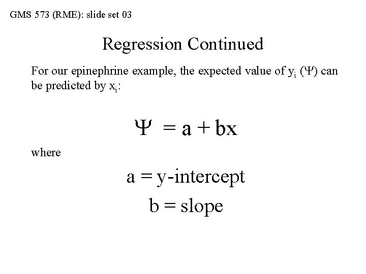
GMS 573 (RME): slide set 03 Regression Continued For our epinephrine example, the expected value of yi ( ) can be predicted by xi: = a + bx where a = y-intercept b = slope

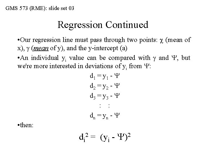
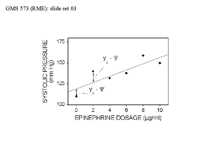
GMS 573 (RME): slide set 03 Regression Continued • Our regression line must pass through two points: (mean of x), (mean of y), and the y-intercept (a) • An individual yi value can be compared with and , but we're more interested in deviations of yi from : d 1 = y 1 - d 2 = y 2 - d 3 = y 3 - : : dn = yn - • then: di 2 = (yi - )2

GMS 573 (RME): slide set 03

GMS 573 (RME): slide set 03

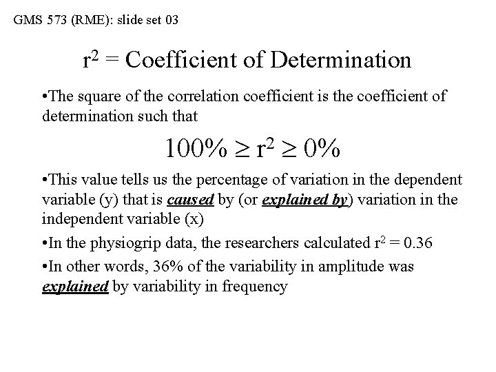
GMS 573 (RME): slide set 03 r 2 = Coefficient of Determination • The square of the correlation coefficient is the coefficient of determination such that 100% r 2 0% • This value tells us the percentage of variation in the dependent variable (y) that is caused by (or explained by) variation in the independent variable (x) • In the physiogrip data, the researchers calculated r 2 = 0. 36 • In other words, 36% of the variability in amplitude was explained by variability in frequency

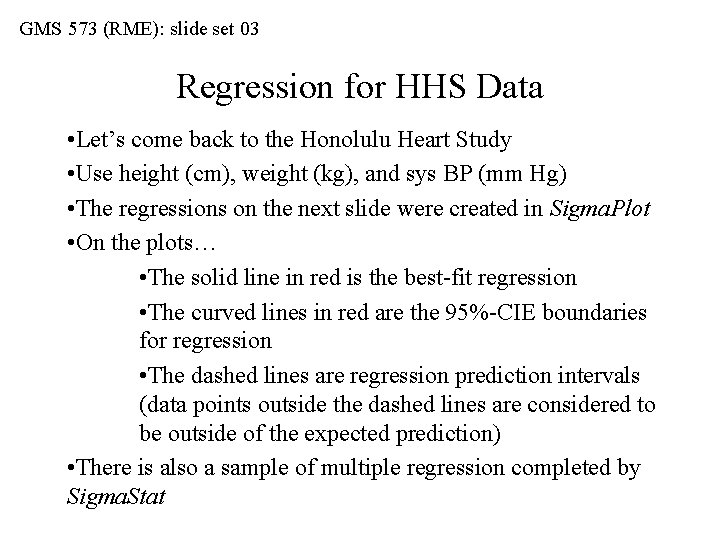
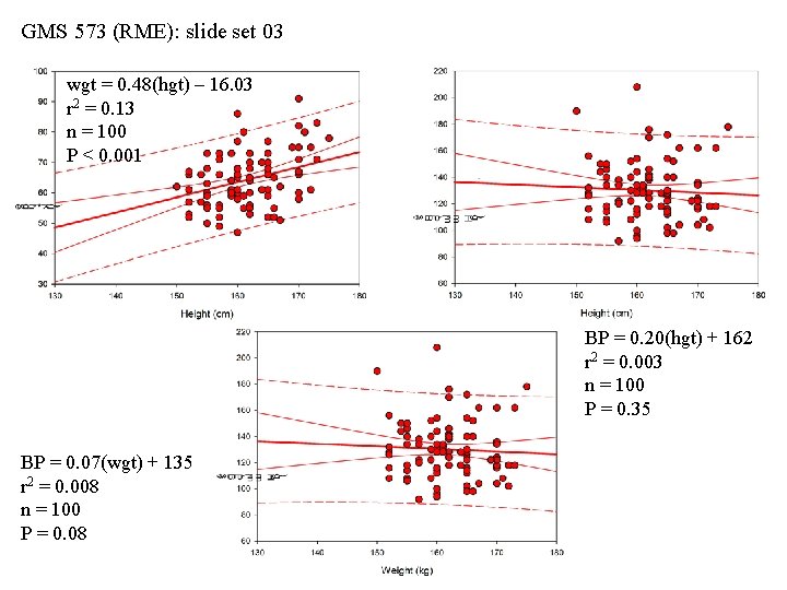
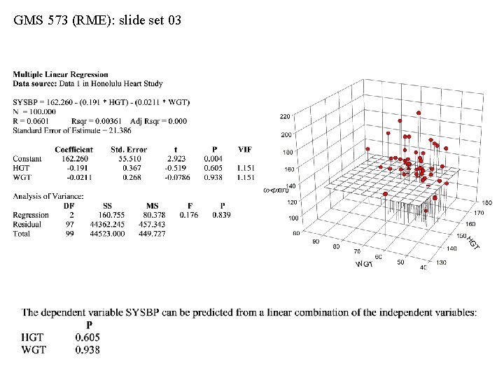
GMS 573 (RME): slide set 03 Regression for HHS Data • Let’s come back to the Honolulu Heart Study • Use height (cm), weight (kg), and sys BP (mm Hg) • The regressions on the next slide were created in Sigma. Plot • On the plots… • The solid line in red is the best-fit regression • The curved lines in red are the 95%-CIE boundaries for regression • The dashed lines are regression prediction intervals (data points outside the dashed lines are considered to be outside of the expected prediction) • There is also a sample of multiple regression completed by Sigma. Stat

GMS 573 (RME): slide set 03 wgt = 0. 48(hgt) – 16. 03 r 2 = 0. 13 n = 100 P < 0. 001 BP = 0. 20(hgt) + 162 r 2 = 0. 003 n = 100 P = 0. 35 BP = 0. 07(wgt) + 135 r 2 = 0. 008 n = 100 P = 0. 08

GMS 573 (RME): slide set 03

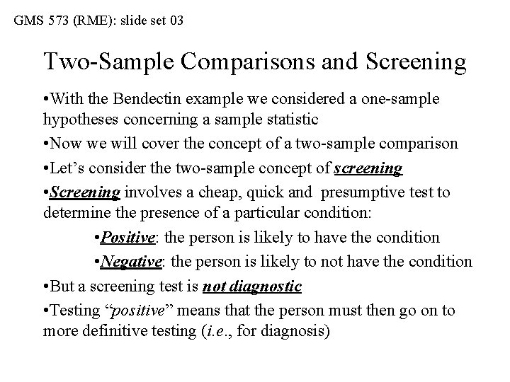
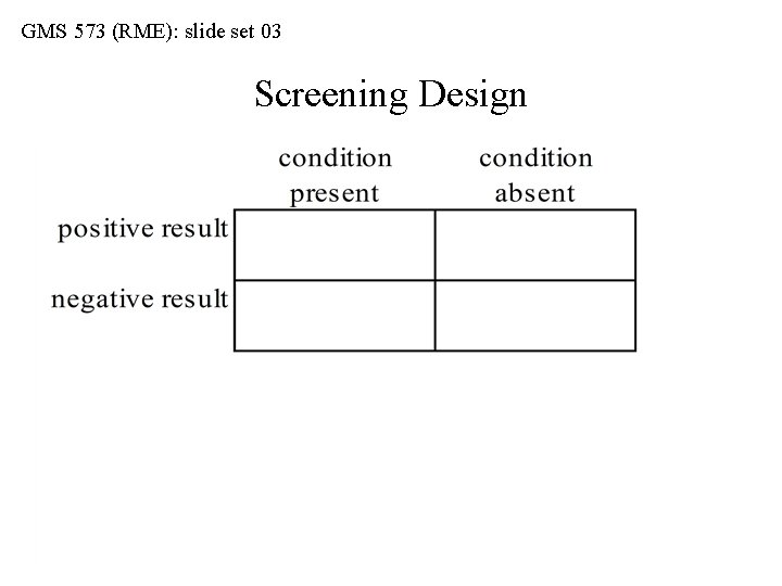
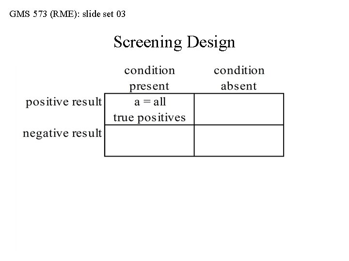
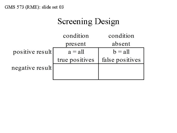
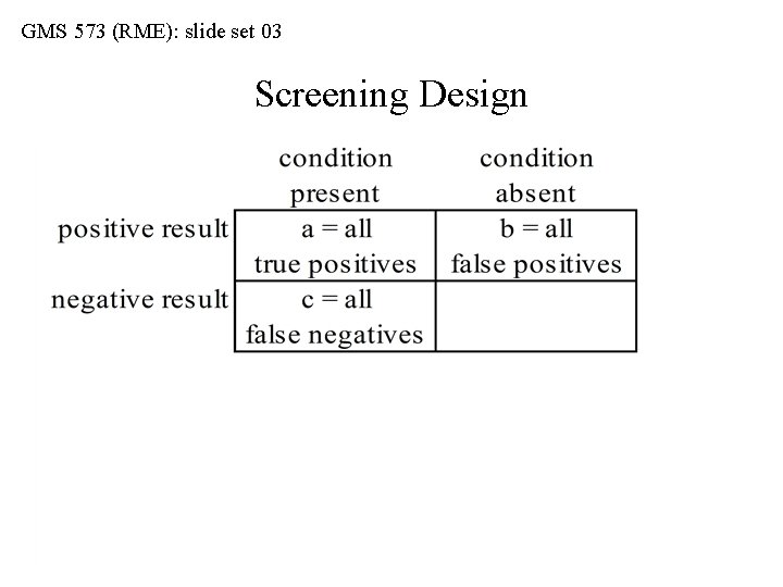
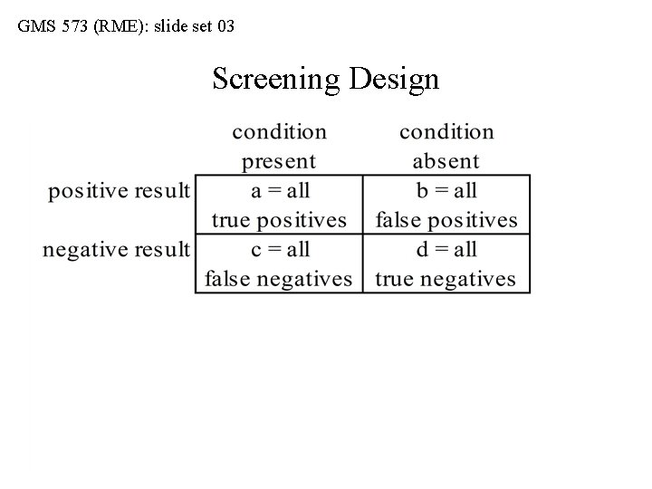
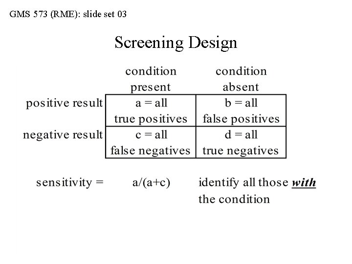
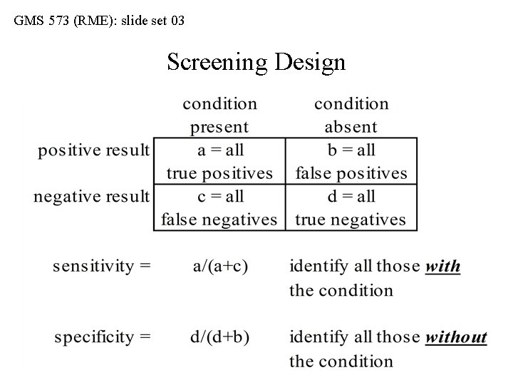
GMS 573 (RME): slide set 03 Two-Sample Comparisons and Screening • With the Bendectin example we considered a one-sample hypotheses concerning a sample statistic • Now we will cover the concept of a two-sample comparison • Let’s consider the two-sample concept of screening • Screening involves a cheap, quick and presumptive test to determine the presence of a particular condition: • Positive: the person is likely to have the condition • Negative: the person is likely to not have the condition • But a screening test is not diagnostic • Testing “positive” means that the person must then go on to more definitive testing (i. e. , for diagnosis)

GMS 573 (RME): slide set 03 Screening Design

GMS 573 (RME): slide set 03 Screening Design

GMS 573 (RME): slide set 03 Screening Design

GMS 573 (RME): slide set 03 Screening Design

GMS 573 (RME): slide set 03 Screening Design

GMS 573 (RME): slide set 03 Screening Design

GMS 573 (RME): slide set 03 Screening Design

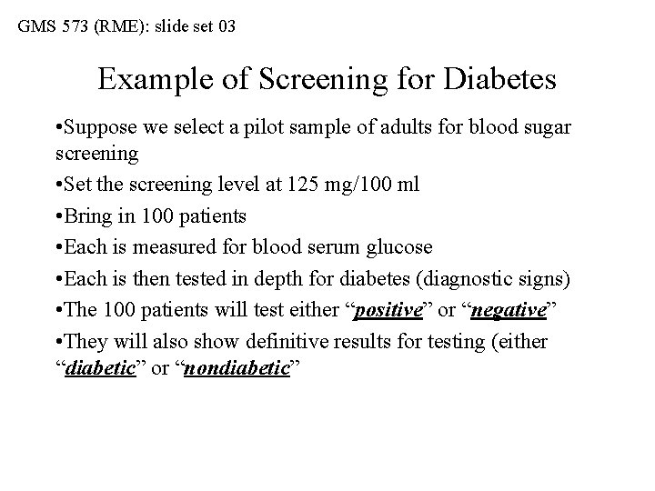
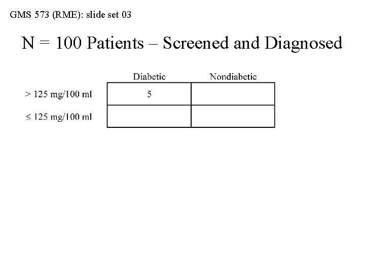
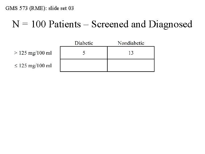
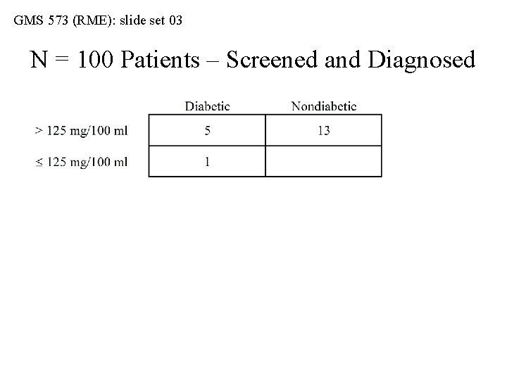
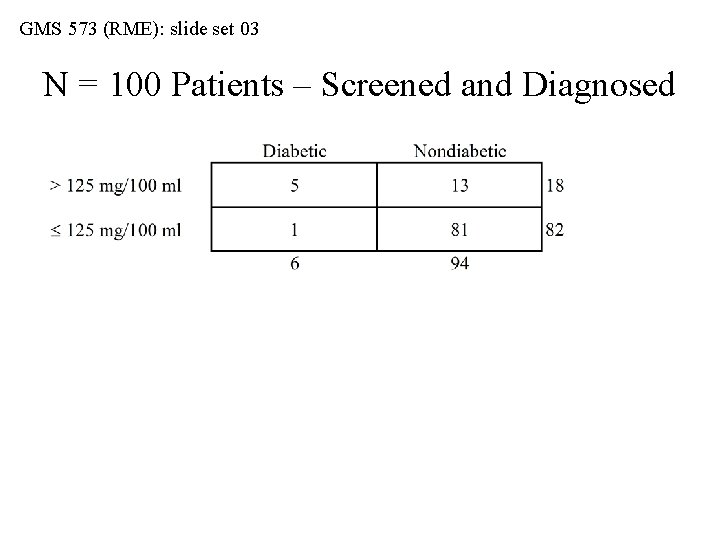
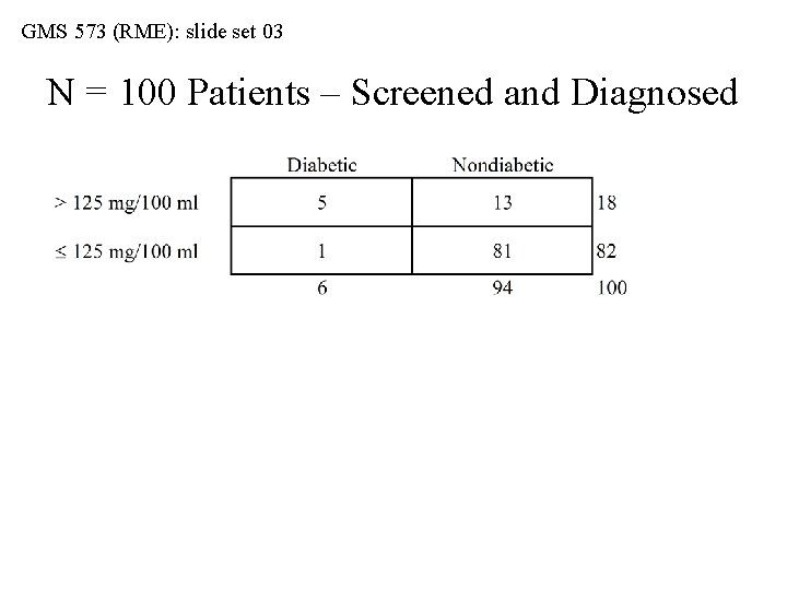
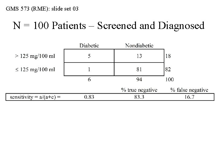
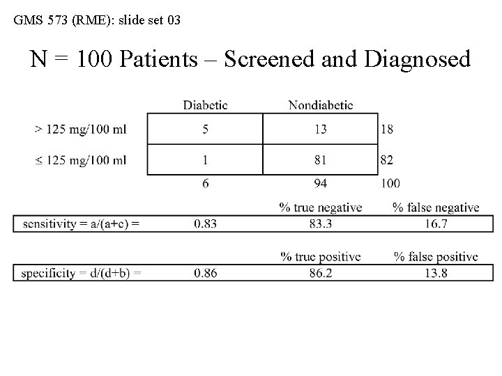
GMS 573 (RME): slide set 03 Example of Screening for Diabetes • Suppose we select a pilot sample of adults for blood sugar screening • Set the screening level at 125 mg/100 ml • Bring in 100 patients • Each is measured for blood serum glucose • Each is then tested in depth for diabetes (diagnostic signs) • The 100 patients will test either “positive” or “negative” • They will also show definitive results for testing (either “diabetic” or “nondiabetic”

GMS 573 (RME): slide set 03 N = 100 Patients – Screened and Diagnosed

GMS 573 (RME): slide set 03 N = 100 Patients – Screened and Diagnosed

GMS 573 (RME): slide set 03 N = 100 Patients – Screened and Diagnosed

GMS 573 (RME): slide set 03 N = 100 Patients – Screened and Diagnosed

GMS 573 (RME): slide set 03 N = 100 Patients – Screened and Diagnosed

GMS 573 (RME): slide set 03 N = 100 Patients – Screened and Diagnosed

GMS 573 (RME): slide set 03 N = 100 Patients – Screened and Diagnosed

GMS 573 (RME): slide set 03 N = 100 Patients – Screened and Diagnosed

GMS 573 (RME): slide set 03 N = 100 Patients – Screened and Diagnosed

GMS 573 (RME): slide set 03 N = 100 Patients – Screened and Diagnosed

GMS 573 (RME): slide set 03 N = 100 Patients – Screened and Diagnosed

GMS 573 (RME): slide set 03 N = 100 Patients – Screened and Diagnosed

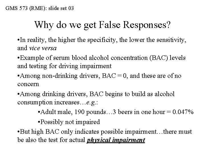
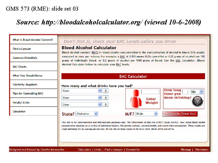
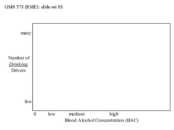
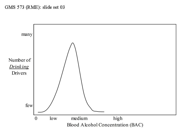
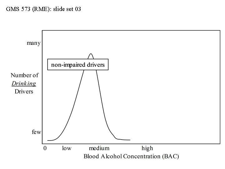
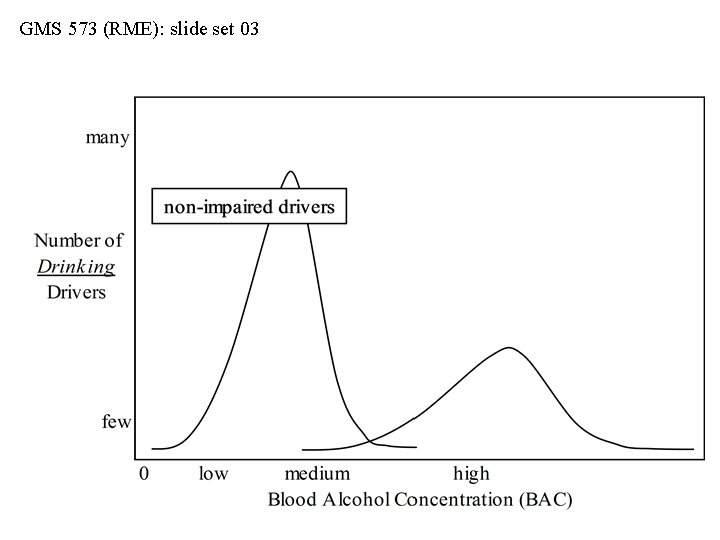
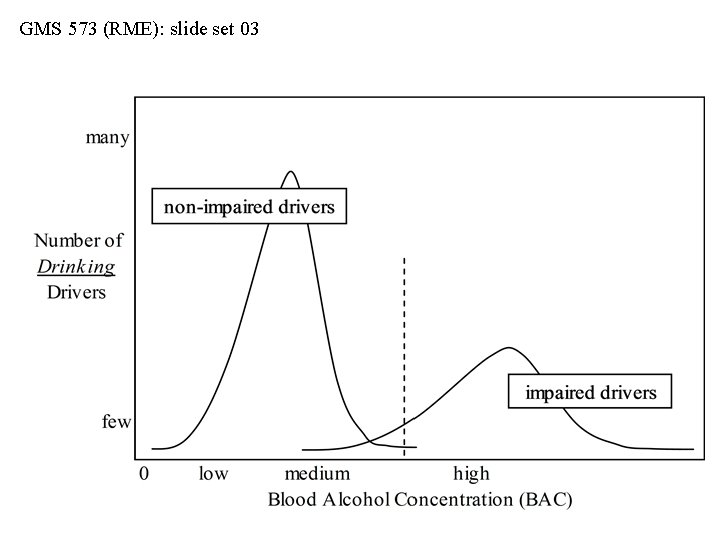
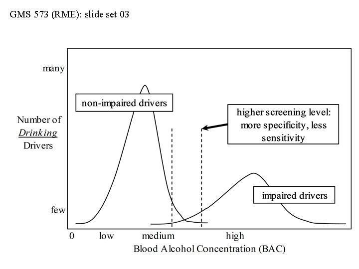
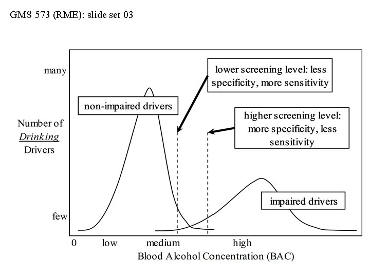
GMS 573 (RME): slide set 03 Why do we get False Responses? • In reality, the higher the specificity, the lower the sensitivity, and vice versa • Example of serum blood alcohol concentration (BAC) levels and testing for driving impairment • Among non-drinking drivers, BAC = 0, and these are of no concern • Among drinking drivers, BAC begins to build as alcohol consumption increases…e. g. : • Adult male, 190 pounds… 3 beers in one hour = 0. 047% • Possibly not impaired • But high BAC only indicates possible impairment…there must be also the test for actual physical impairment

GMS 573 (RME): slide set 03 Source: http: //bloodalcoholcalculator. org/ (viewed 10 -6 -2008)

GMS 573 (RME): slide set 03

GMS 573 (RME): slide set 03

GMS 573 (RME): slide set 03

GMS 573 (RME): slide set 03

GMS 573 (RME): slide set 03

GMS 573 (RME): slide set 03

GMS 573 (RME): slide set 03

GMS 573 (RME): slide set 03

GMS 573 (RME): slide set 03

GMS 573 (RME): slide set 03 Other Two-Sample Hypotheses • Another approach in two-sample hypotheses concerns the comparison of sample means • This is a broad area in so-called “parametric” statistics (i. e. , methods using sample means and sample standard deviations) • Most of these methods concern so-called “t-testing” and “analysis of variance” (so-called “ANOVA”) • So-called “non-parametric” statistics include the two-sample comparison of proportions of qualitative states (not means), e. g. , percent “heads” vs. percent “tails” in coin flips…this approach is more suitable for co-called “Chi-Square” methods • For a simple two-sample comparison of means I will use only the comparison of 95%-CIE intervals

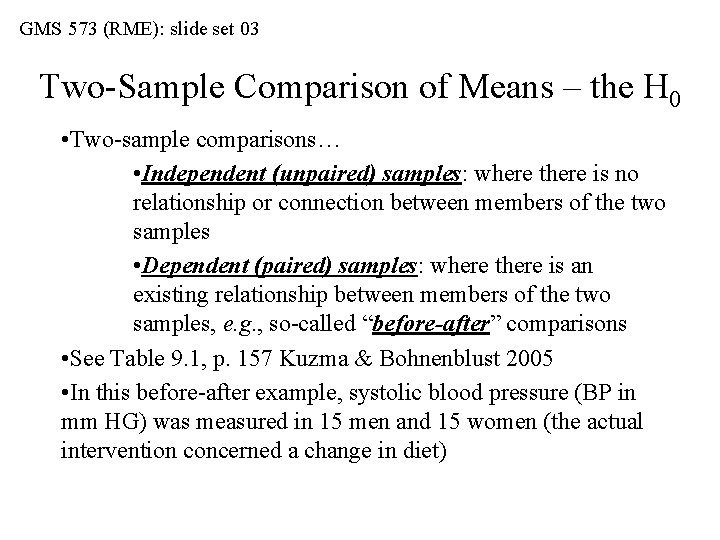
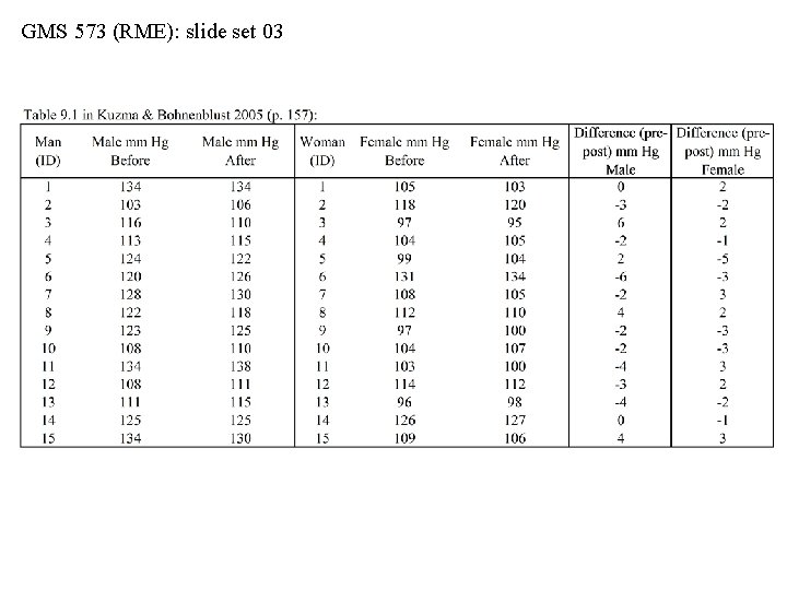
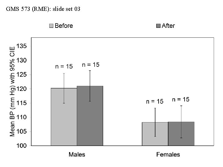
GMS 573 (RME): slide set 03 Two-Sample Comparison of Means – the H 0 • Two-sample comparisons… • Independent (unpaired) samples: where there is no relationship or connection between members of the two samples • Dependent (paired) samples: where there is an existing relationship between members of the two samples, e. g. , so-called “before-after” comparisons • See Table 9. 1, p. 157 Kuzma & Bohnenblust 2005 • In this before-after example, systolic blood pressure (BP in mm HG) was measured in 15 men and 15 women (the actual intervention concerned a change in diet)

GMS 573 (RME): slide set 03

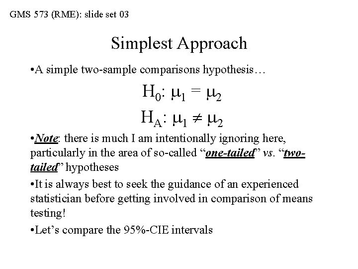
GMS 573 (RME): slide set 03 Simplest Approach • A simple two-sample comparisons hypothesis… H 0: 1 = 2 H A: 1 2 • Note: there is much I am intentionally ignoring here, particularly in the area of so-called “one-tailed” vs. “twotailed” hypotheses • It is always best to seek the guidance of an experienced statistician before getting involved in comparison of means testing! • Let’s compare the 95%-CIE intervals

GMS 573 (RME): slide set 03