Example 16 1 Calculating the p H of

Example 16. 1 Calculating the p. H of a Buffer Solution Calculate the p. H of a buffer solution that is 0. 100 M in HC 2 H 3 O 2 and 0. 100 M in Na. C 2 H 3 O 2 Solution 1. Write the balanced equation for the ionization of the acid and use it as a guide to prepare an ICE table showing the given concentrations of the acid and its conjugate base as the initial concentrations. Leave room in the table for the changes in concentrations and for the equilibrium concentrations. 2. Represent the change in the concentration of H 3 O+ with the variable x. Express the changes in the concentrations of the other reactants and products in terms of x. Chemistry: A Molecular Approach, 3 rd Edition Nivaldo J. Tro © 2014 Pearson Education, Inc.

Example 16. 1 Calculating the p. H of a Buffer Solution Continued 3. Sum each column to determine the equilibrium concentrations in terms of the initial concentrations and the variable x. 4. Substitute the expressions for the equilibrium concentrations (from step 3) into the expression for the acid ionization constant. In most cases, you can make the approximation that x is small. (See Sections 14. 8 and 15. 6 to review the x is small approximation. ) Chemistry: A Molecular Approach, 3 rd Edition Nivaldo J. Tro © 2014 Pearson Education, Inc.

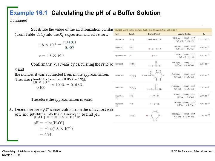
Example 16. 1 Calculating the p. H of a Buffer Solution Continued Substitute the value of the acid ionization constant (from Table 15. 5) into the Ka expression and solve for x. Confirm that x is small by calculating the ratio of x and the number it was subtracted from in the approximation. The ratio should be less than 0. 05 (or 5%). Therefore the approximation is valid. 5. Determine the H 3 O+ concentration from the calculated value of x and substitute into the p. H equation to find p. H. Chemistry: A Molecular Approach, 3 rd Edition Nivaldo J. Tro © 2014 Pearson Education, Inc.

Example 16. 1 Calculating the p. H of a Buffer Solution Continued For Practice 16. 1 Calculate the p. H of a buffer solution that is 0. 200 M in HC 2 H 3 O 2 and 0. 100 M in Na. C 2 H 3 O 2. For More Practice 16. 1 Calculate the p. H of the buffer that results from mixing 60. 0 m. L of 0. 250 M HCHO 2 and 15. 0 m. L of 0. 500 M Na. CHO 2. Chemistry: A Molecular Approach, 3 rd Edition Nivaldo J. Tro © 2014 Pearson Education, Inc.

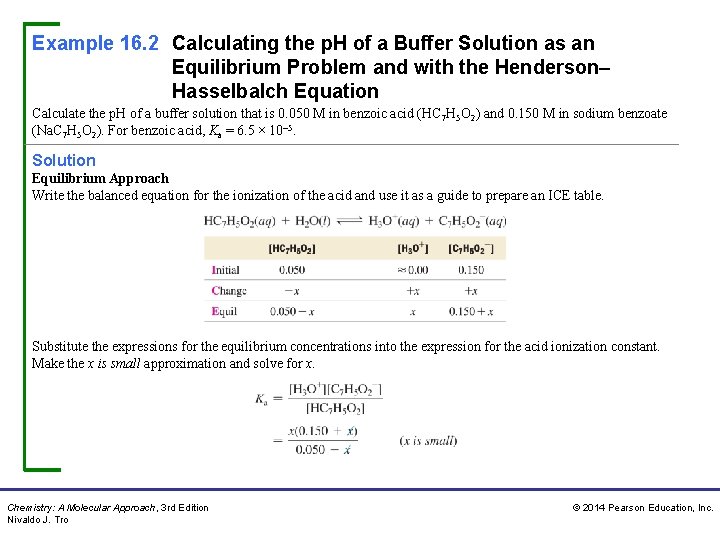
Example 16. 2 Calculating the p. H of a Buffer Solution as an Equilibrium Problem and with the Henderson– Hasselbalch Equation Calculate the p. H of a buffer solution that is 0. 050 M in benzoic acid (HC 7 H 5 O 2) and 0. 150 M in sodium benzoate (Na. C 7 H 5 O 2). For benzoic acid, Ka = 6. 5 × 10– 5. Solution Equilibrium Approach Write the balanced equation for the ionization of the acid and use it as a guide to prepare an ICE table. Substitute the expressions for the equilibrium concentrations into the expression for the acid ionization constant. Make the x is small approximation and solve for x. Chemistry: A Molecular Approach, 3 rd Edition Nivaldo J. Tro © 2014 Pearson Education, Inc.

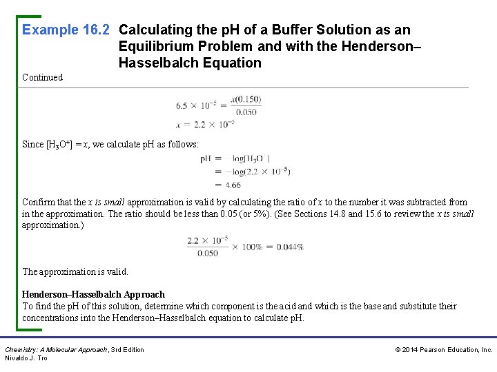
Example 16. 2 Calculating the p. H of a Buffer Solution as an Equilibrium Problem and with the Henderson– Hasselbalch Equation Continued Since [H 3 O+] = x, we calculate p. H as follows: Confirm that the x is small approximation is valid by calculating the ratio of x to the number it was subtracted from in the approximation. The ratio should be less than 0. 05 (or 5%). (See Sections 14. 8 and 15. 6 to review the x is small approximation. ) The approximation is valid. Henderson–Hasselbalch Approach To find the p. H of this solution, determine which component is the acid and which is the base and substitute their concentrations into the Henderson–Hasselbalch equation to calculate p. H. Chemistry: A Molecular Approach, 3 rd Edition Nivaldo J. Tro © 2014 Pearson Education, Inc.

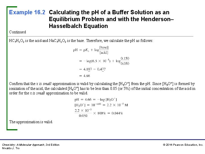
Example 16. 2 Calculating the p. H of a Buffer Solution as an Equilibrium Problem and with the Henderson– Hasselbalch Equation Continued HC 7 H 5 O 2 is the acid and Na. C 7 H 5 O 2 is the base. Therefore, we calculate the p. H as follows: Confirm that the x is small approximation is valid by calculating the [H 3 O+] from the p. H. Since [H 3 O+] is formed by ionization of the acid, the calculated [H 3 O+] has to be less than 0. 05 (or 5%) of the initial concentration of the acid in order for the x is small approximation to be valid. The approximation is valid. Chemistry: A Molecular Approach, 3 rd Edition Nivaldo J. Tro © 2014 Pearson Education, Inc.

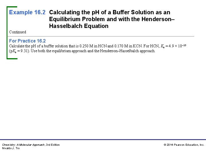
Example 16. 2 Calculating the p. H of a Buffer Solution as an Equilibrium Problem and with the Henderson– Hasselbalch Equation Continued For Practice 16. 2 Calculate the p. H of a buffer solution that is 0. 250 M in HCN and 0. 170 M in KCN. For HCN, Ka = 4. 9 × 10– 10 (p. Ka = 9. 31). Use both the equilibrium approach and the Henderson–Hasselbalch approach. Chemistry: A Molecular Approach, 3 rd Edition Nivaldo J. Tro © 2014 Pearson Education, Inc.

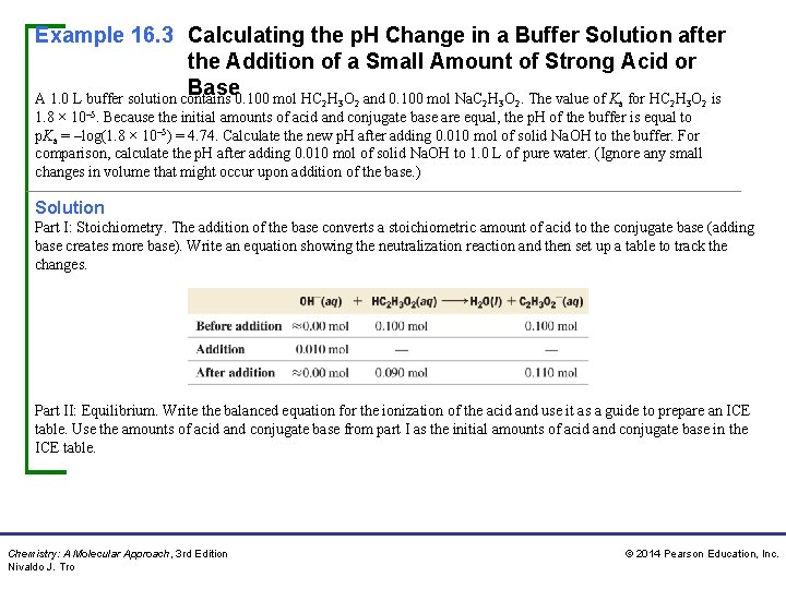
Example 16. 3 Calculating the p. H Change in a Buffer Solution after the Addition of a Small Amount of Strong Acid or Base A 1. 0 L buffer solution contains 0. 100 mol HC H O and 0. 100 mol Na. C H O. The value of K for HC H O is 2 3 2 a 2 3 2 1. 8 × 10– 5. Because the initial amounts of acid and conjugate base are equal, the p. H of the buffer is equal to p. Ka = –log(1. 8 × 10– 5) = 4. 74. Calculate the new p. H after adding 0. 010 mol of solid Na. OH to the buffer. For comparison, calculate the p. H after adding 0. 010 mol of solid Na. OH to 1. 0 L of pure water. (Ignore any small changes in volume that might occur upon addition of the base. ) Solution Part I: Stoichiometry. The addition of the base converts a stoichiometric amount of acid to the conjugate base (adding base creates more base). Write an equation showing the neutralization reaction and then set up a table to track the changes. Part II: Equilibrium. Write the balanced equation for the ionization of the acid and use it as a guide to prepare an ICE table. Use the amounts of acid and conjugate base from part I as the initial amounts of acid and conjugate base in the ICE table. Chemistry: A Molecular Approach, 3 rd Edition Nivaldo J. Tro © 2014 Pearson Education, Inc.

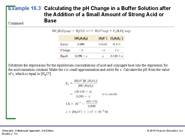
Example 16. 3 Calculating the p. H Change in a Buffer Solution after the Addition of a Small Amount of Strong Acid or Base Continued Substitute the expressions for the equilibrium concentrations of acid and conjugate base into the expression for the acid ionization constant. Make the x is small approximation and solve for x. Calculate the p. H from the value of x, which is equal to [H 3 O+]. Chemistry: A Molecular Approach, 3 rd Edition Nivaldo J. Tro © 2014 Pearson Education, Inc.

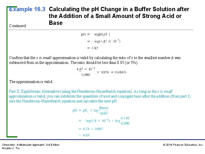
Example 16. 3 Calculating the p. H Change in a Buffer Solution after the Addition of a Small Amount of Strong Acid or Base Continued Confirm that the x is small approximation is valid by calculating the ratio of x to the smallest number it was subtracted from in the approximation. The ratio should be less than 0. 05 (or 5%). The approximation is valid. Part II: Equilibrium Alternative (using the Henderson–Hasselbalch equation). As long as the x is small approximation is valid, you can substitute the quantities of acid and conjugate base after the addition (from part I) into the Henderson–Hasselbalch equation and calculate the new p. H. Chemistry: A Molecular Approach, 3 rd Edition Nivaldo J. Tro © 2014 Pearson Education, Inc.

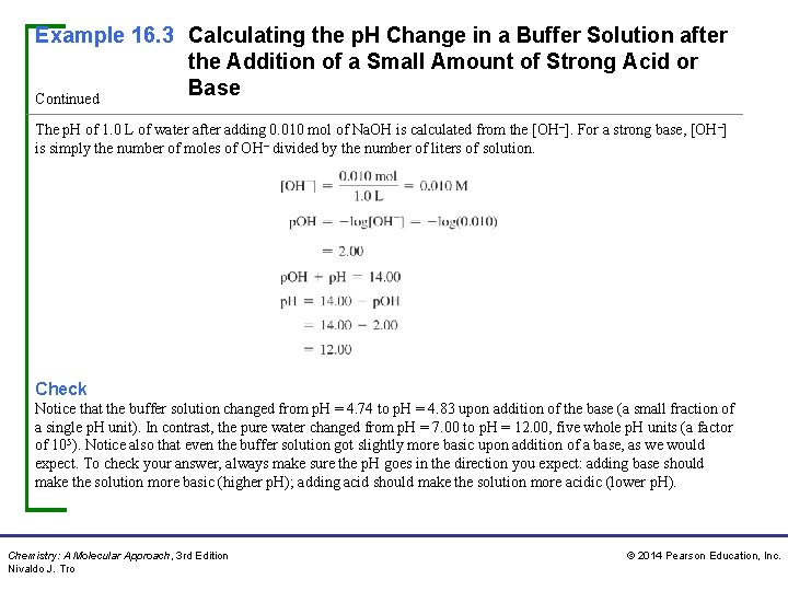
Example 16. 3 Calculating the p. H Change in a Buffer Solution after the Addition of a Small Amount of Strong Acid or Base Continued The p. H of 1. 0 L of water after adding 0. 010 mol of Na. OH is calculated from the [OH–]. For a strong base, [OH–] is simply the number of moles of OH– divided by the number of liters of solution. Check Notice that the buffer solution changed from p. H = 4. 74 to p. H = 4. 83 upon addition of the base (a small fraction of a single p. H unit). In contrast, the pure water changed from p. H = 7. 00 to p. H = 12. 00, five whole p. H units (a factor of 105). Notice also that even the buffer solution got slightly more basic upon addition of a base, as we would expect. To check your answer, always make sure the p. H goes in the direction you expect: adding base should make the solution more basic (higher p. H); adding acid should make the solution more acidic (lower p. H). Chemistry: A Molecular Approach, 3 rd Edition Nivaldo J. Tro © 2014 Pearson Education, Inc.

Example 16. 3 Calculating the p. H Change in a Buffer Solution after the Addition of a Small Amount of Strong Acid or Base Continued For Practice 16. 3 Calculate the p. H of the solution in Example 16. 3 upon addition of 0. 015 mol of Na. OH to the original buffer. For More Practice 16. 3 Calculate the p. H of the solution in Example 16. 3 upon addition of 10. 0 m. L of 1. 00 M HCl to the original buffer in Example 16. 3. Chemistry: A Molecular Approach, 3 rd Edition Nivaldo J. Tro © 2014 Pearson Education, Inc.

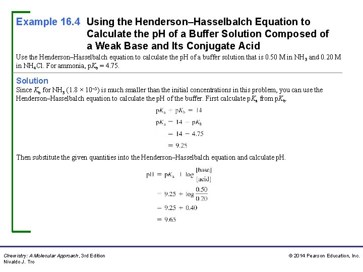
Example 16. 4 Using the Henderson–Hasselbalch Equation to Calculate the p. H of a Buffer Solution Composed of a Weak Base and Its Conjugate Acid Use the Henderson–Hasselbalch equation to calculate the p. H of a buffer solution that is 0. 50 M in NH 3 and 0. 20 M in NH 4 Cl. For ammonia, p. Kb = 4. 75. Solution Since Kb for NH 3 (1. 8 × 10– 5) is much smaller than the initial concentrations in this problem, you can use the Henderson–Hasselbalch equation to calculate the p. H of the buffer. First calculate p. Ka from p. Kb. Then substitute the given quantities into the Henderson–Hasselbalch equation and calculate p. H. Chemistry: A Molecular Approach, 3 rd Edition Nivaldo J. Tro © 2014 Pearson Education, Inc.

Example 16. 4 Using the Henderson–Hasselbalch Equation to Calculate the p. H of a Buffer Solution Composed of a Weak Base and Its Conjugate Acid Continued For Practice 16. 4 Calculate the p. H of 1. 0 L of the solution in Example 16. 4 upon addition of 0. 010 mol of solid Na. OH to the original buffer solution. For More Practice 16. 4 Calculate the p. H of 1. 0 L of the solution in Example 16. 4 upon addition of 30. 0 m. L of 1. 0 M HCl to the original buffer solution. Chemistry: A Molecular Approach, 3 rd Edition Nivaldo J. Tro © 2014 Pearson Education, Inc.

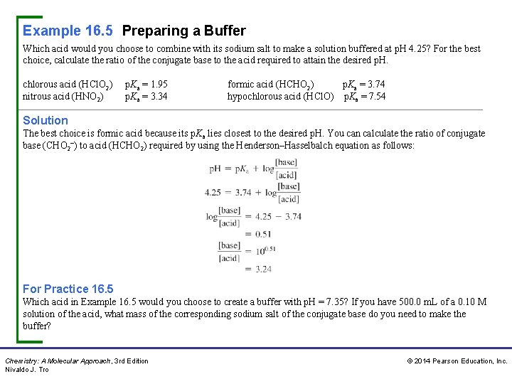
Example 16. 5 Preparing a Buffer Which acid would you choose to combine with its sodium salt to make a solution buffered at p. H 4. 25? For the best choice, calculate the ratio of the conjugate base to the acid required to attain the desired p. H. chlorous acid (HCl. O 2) nitrous acid (HNO 2) p. Ka = 1. 95 p. Ka = 3. 34 formic acid (HCHO 2) p. Ka = 3. 74 hypochlorous acid (HCl. O) p. Ka = 7. 54 Solution The best choice is formic acid because its p. Ka lies closest to the desired p. H. You can calculate the ratio of conjugate base (CHO 2–) to acid (HCHO 2) required by using the Henderson–Hasselbalch equation as follows: For Practice 16. 5 Which acid in Example 16. 5 would you choose to create a buffer with p. H = 7. 35? If you have 500. 0 m. L of a 0. 10 M solution of the acid, what mass of the corresponding sodium salt of the conjugate base do you need to make the buffer? Chemistry: A Molecular Approach, 3 rd Edition Nivaldo J. Tro © 2014 Pearson Education, Inc.

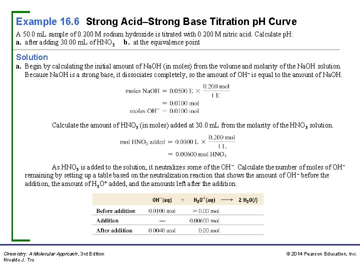
Example 16. 6 Strong Acid–Strong Base Titration p. H Curve A 50. 0 m. L sample of 0. 200 M sodium hydroxide is titrated with 0. 200 M nitric acid. Calculate p. H: a. after adding 30. 00 m. L of HNO 3 b. at the equivalence point Solution a. Begin by calculating the initial amount of Na. OH (in moles) from the volume and molarity of the Na. OH solution. Because Na. OH is a strong base, it dissociates completely, so the amount of OH– is equal to the amount of Na. OH. Calculate the amount of HNO 3 (in moles) added at 30. 0 m. L from the molarity of the HNO 3 solution. As HNO 3 is added to the solution, it neutralizes some of the OH–. Calculate the number of moles of OH– remaining by setting up a table based on the neutralization reaction that shows the amount of OH – before the addition, the amount of H 3 O+ added, and the amounts left after the addition. Chemistry: A Molecular Approach, 3 rd Edition Nivaldo J. Tro © 2014 Pearson Education, Inc.

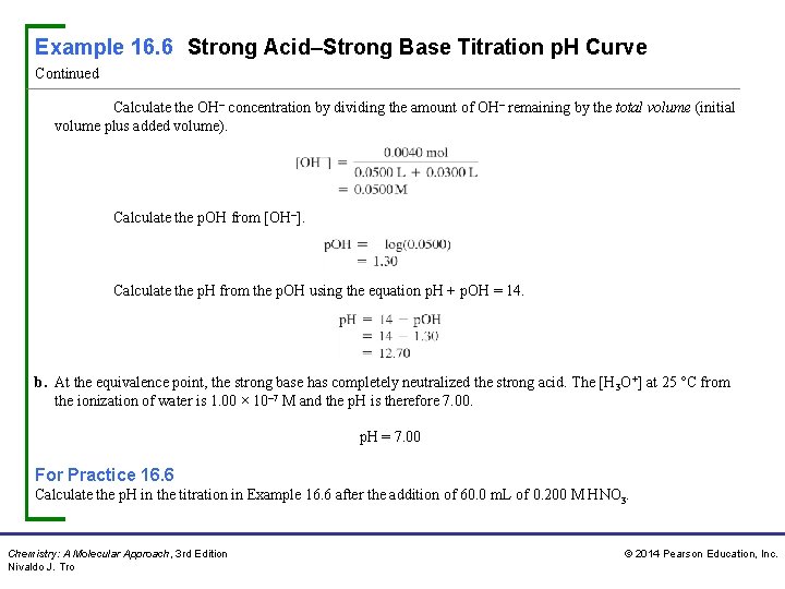
Example 16. 6 Strong Acid–Strong Base Titration p. H Curve Continued Calculate the OH– concentration by dividing the amount of OH– remaining by the total volume (initial volume plus added volume). Calculate the p. OH from [OH–]. Calculate the p. H from the p. OH using the equation p. H + p. OH = 14. b. At the equivalence point, the strong base has completely neutralized the strong acid. The [H 3 O+] at 25 °C from the ionization of water is 1. 00 × 10– 7 M and the p. H is therefore 7. 00. p. H = 7. 00 For Practice 16. 6 Calculate the p. H in the titration in Example 16. 6 after the addition of 60. 0 m. L of 0. 200 M HNO 3. Chemistry: A Molecular Approach, 3 rd Edition Nivaldo J. Tro © 2014 Pearson Education, Inc.

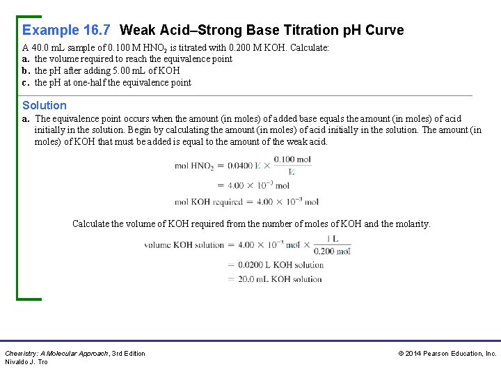
Example 16. 7 Weak Acid–Strong Base Titration p. H Curve A 40. 0 m. L sample of 0. 100 M HNO 2 is titrated with 0. 200 M KOH. Calculate: a. the volume required to reach the equivalence point b. the p. H after adding 5. 00 m. L of KOH c. the p. H at one-half the equivalence point Solution a. The equivalence point occurs when the amount (in moles) of added base equals the amount (in moles) of acid initially in the solution. Begin by calculating the amount (in moles) of acid initially in the solution. The amount (in moles) of KOH that must be added is equal to the amount of the weak acid. Calculate the volume of KOH required from the number of moles of KOH and the molarity. Chemistry: A Molecular Approach, 3 rd Edition Nivaldo J. Tro © 2014 Pearson Education, Inc.

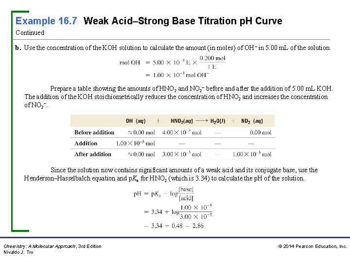
Example 16. 7 Weak Acid–Strong Base Titration p. H Curve Continued b. Use the concentration of the KOH solution to calculate the amount (in moles) of OH– in 5. 00 m. L of the solution. Prepare a table showing the amounts of HNO 2 and NO 2– before and after the addition of 5. 00 m. L KOH. The addition of the KOH stoichiometrically reduces the concentration of HNO 2 and increases the concentration of NO 2–. Since the solution now contains significant amounts of a weak acid and its conjugate base, use the Henderson–Hasselbalch equation and p. Ka for HNO 2 (which is 3. 34) to calculate the p. H of the solution. Chemistry: A Molecular Approach, 3 rd Edition Nivaldo J. Tro © 2014 Pearson Education, Inc.

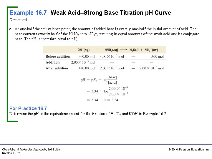
Example 16. 7 Weak Acid–Strong Base Titration p. H Curve Continued c. At one-half the equivalence point, the amount of added base is exactly one-half the initial amount of acid. The base converts exactly half of the HNO 2 into NO 2–, resulting in equal amounts of the weak acid and its conjugate base. The p. H is therefore equal to p. Ka. For Practice 16. 7 Determine the p. H at the equivalence point for the titration of HNO 2 and KOH in Example 16. 7. Chemistry: A Molecular Approach, 3 rd Edition Nivaldo J. Tro © 2014 Pearson Education, Inc.

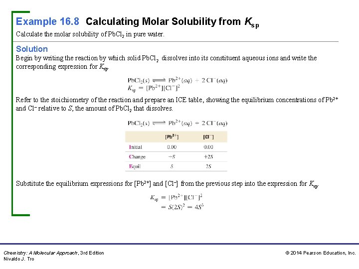
Example 16. 8 Calculating Molar Solubility from Ksp Calculate the molar solubility of Pb. Cl 2 in pure water. Solution Begin by writing the reaction by which solid Pb. Cl 2 dissolves into its constituent aqueous ions and write the corresponding expression for Ksp. Refer to the stoichiometry of the reaction and prepare an ICE table, showing the equilibrium concentrations of Pb 2+ and Cl– relative to S, the amount of Pb. Cl 2 that dissolves. Substitute the equilibrium expressions for [Pb 2+] and [Cl–] from the previous step into the expression for Ksp. Chemistry: A Molecular Approach, 3 rd Edition Nivaldo J. Tro © 2014 Pearson Education, Inc.

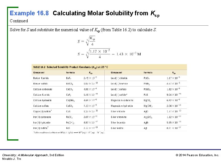
Example 16. 8 Calculating Molar Solubility from Ksp Continued Solve for S and substitute the numerical value of Ksp (from Table 16. 2) to calculate S. Chemistry: A Molecular Approach, 3 rd Edition Nivaldo J. Tro © 2014 Pearson Education, Inc.

Example 16. 8 Calculating Molar Solubility from Ksp Continued For Practice 16. 8 Calculate the molar solubility of Fe(OH)2 in pure water. Chemistry: A Molecular Approach, 3 rd Edition Nivaldo J. Tro © 2014 Pearson Education, Inc.

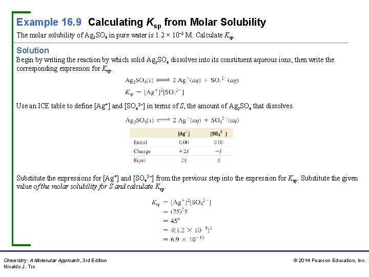
Example 16. 9 Calculating Ksp from Molar Solubility The molar solubility of Ag 2 SO 4 in pure water is 1. 2 × 10– 5 M. Calculate Ksp. Solution Begin by writing the reaction by which solid Ag 2 SO 4 dissolves into its constituent aqueous ions, then write the corresponding expression for Ksp. Use an ICE table to define [Ag+] and [SO 42–] in terms of S, the amount of Ag 2 SO 4 that dissolves. Substitute the expressions for [Ag+] and [SO 42–] from the previous step into the expression for Ksp. Substitute the given value of the molar solubility for S and calculate Ksp. Chemistry: A Molecular Approach, 3 rd Edition Nivaldo J. Tro © 2014 Pearson Education, Inc.

Example 16. 9 Calculating Ksp from Molar Solubility Continued For Practice 16. 9 The molar solubility of Ag. Br in pure water is 7. 3 × 10– 7 M. Calculate Ksp. Chemistry: A Molecular Approach, 3 rd Edition Nivaldo J. Tro © 2014 Pearson Education, Inc.

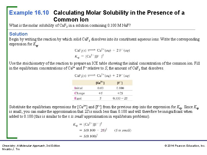
Example 16. 10 Calculating Molar Solubility in the Presence of a Common Ion What is the molar solubility of Ca. F 2 in a solution containing 0. 100 M Na. F? Solution Begin by writing the reaction by which solid Ca. F 2 dissolves into its constituent aqueous ions. Write the corresponding expression for Ksp. Use the stoichiometry of the reaction to prepare an ICE table showing the initial concentration of the common ion. Fill in the equilibrium concentrations of Ca 2+ and F– relative to S, the amount of Ca. F 2 that dissolves. Substitute the equilibrium expressions for [Ca 2+] and [F–] from the previous step into the expression for Ksp. Since Ksp is small, you can make the approximation that 2 S is much less than 0. 100 and will therefore be insignificant when added to 0. 100 (this is similar to the x is small approximation in equilibrium problems). Chemistry: A Molecular Approach, 3 rd Edition Nivaldo J. Tro © 2014 Pearson Education, Inc.

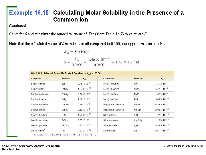
Example 16. 10 Calculating Molar Solubility in the Presence of a Common Ion Continued Solve for S and substitute the numerical value of Ksp (from Table 16. 2) to calculate S. Note that the calculated value of S is indeed small compared to 0. 100; our approximation is valid. Chemistry: A Molecular Approach, 3 rd Edition Nivaldo J. Tro © 2014 Pearson Education, Inc.

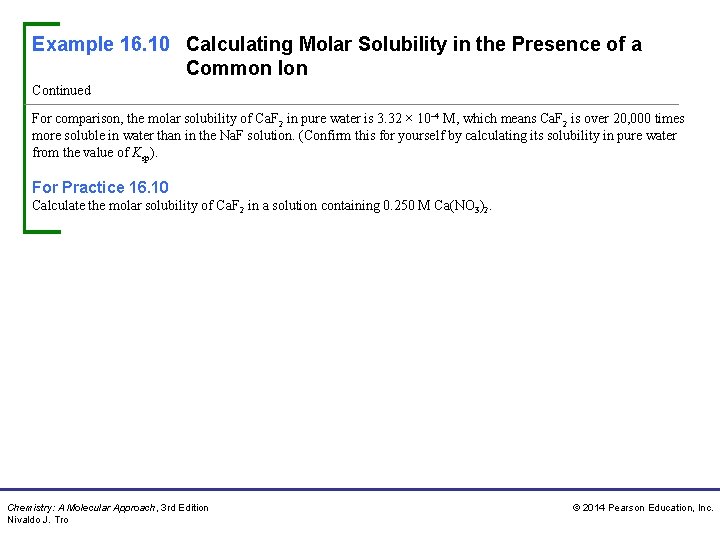
Example 16. 10 Calculating Molar Solubility in the Presence of a Common Ion Continued For comparison, the molar solubility of Ca. F 2 in pure water is 3. 32 × 10– 4 M, which means Ca. F 2 is over 20, 000 times more soluble in water than in the Na. F solution. (Confirm this for yourself by calculating its solubility in pure water from the value of Ksp). For Practice 16. 10 Calculate the molar solubility of Ca. F 2 in a solution containing 0. 250 M Ca(NO 3)2. Chemistry: A Molecular Approach, 3 rd Edition Nivaldo J. Tro © 2014 Pearson Education, Inc.

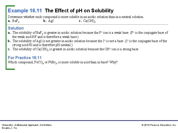
Example 16. 11 The Effect of p. H on Solubility Determine whether each compound is more soluble in an acidic solution than in a neutral solution. a. Ba. F 2 b. Ag. I c. Ca(OH)2 Solution a. The solubility of Ba. F 2 is greater in acidic solution because the F– ion is a weak base. (F– is the conjugate base of the weak acid HF and is therefore a weak base. ) b. The solubility of Ag. I is not greater in acidic solution because the I– is not a base. (I– is the conjugate base of the strong acid HI and is therefore p. H-neutral. ) c. The solubility of Ca(OH)2 is greater in acidic solution because the OH– ion is a strong base. For Practice 16. 11 Which compound, Fe. CO 3 or Pb. Br 2, is more soluble in acid than in base? Why? Chemistry: A Molecular Approach, 3 rd Edition Nivaldo J. Tro © 2014 Pearson Education, Inc.

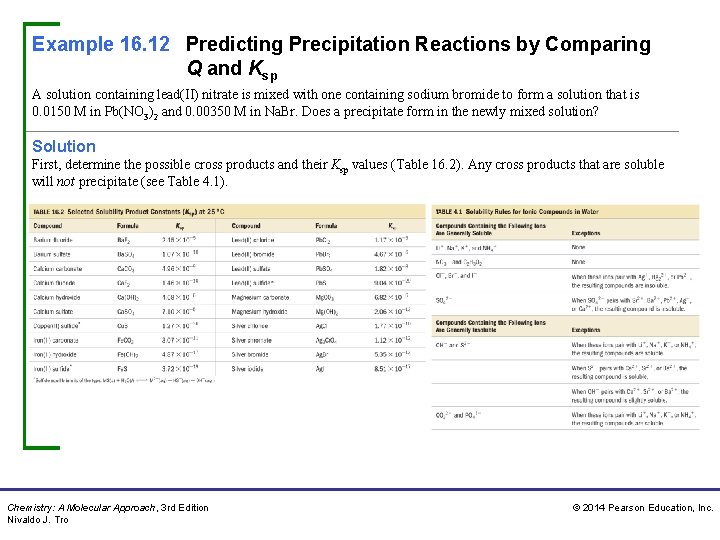
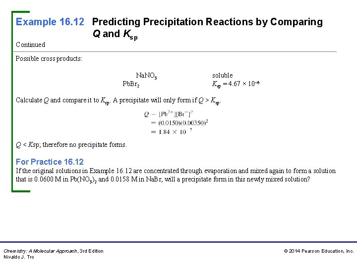
Example 16. 12 Predicting Precipitation Reactions by Comparing Q and Ksp A solution containing lead(II) nitrate is mixed with one containing sodium bromide to form a solution that is 0. 0150 M in Pb(NO 3)2 and 0. 00350 M in Na. Br. Does a precipitate form in the newly mixed solution? Solution First, determine the possible cross products and their Ksp values (Table 16. 2). Any cross products that are soluble will not precipitate (see Table 4. 1). Chemistry: A Molecular Approach, 3 rd Edition Nivaldo J. Tro © 2014 Pearson Education, Inc.

Example 16. 12 Predicting Precipitation Reactions by Comparing Q and Ksp Continued Possible cross products: Na. NO 3 Pb. Br 2 soluble Ksp = 4. 67 × 10– 6 Calculate Q and compare it to Ksp. A precipitate will only form if Q > Ksp. Q < Ksp; therefore no precipitate forms. For Practice 16. 12 If the original solutions in Example 16. 12 are concentrated through evaporation and mixed again to form a solution that is 0. 0600 M in Pb(NO 3)2 and 0. 0158 M in Na. Br, will a precipitate form in this newly mixed solution? Chemistry: A Molecular Approach, 3 rd Edition Nivaldo J. Tro © 2014 Pearson Education, Inc.

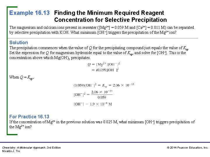
Example 16. 13 Finding the Minimum Required Reagent Concentration for Selective Precipitation The magnesium and calcium ions present in seawater ([Mg 2+] = 0. 059 M and [Ca 2+] = 0. 011 M) can be separated by selective precipitation with KOH. What minimum [OH–] triggers the precipitation of the Mg 2+ ion? Solution The precipitation commences when the value of Q for the precipitating compound just equals the value of Ksp. Set the expression for Q for magnesium hydroxide equal to the value of Ksp, and solve for [OH–]. This is the concentration above which Mg(OH)2 precipitates. When Q = Ksp, For Practice 16. 13 If the concentration of Mg 2+ in the previous solution was 0. 025 M, what minimum [OH–] triggers precipitation of the Mg 2+ ion? Chemistry: A Molecular Approach, 3 rd Edition Nivaldo J. Tro © 2014 Pearson Education, Inc.

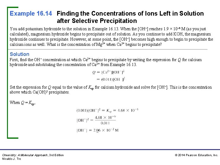
Example 16. 14 Finding the Concentrations of Ions Left in Solution after Selective Precipitation You add potassium hydroxide to the solution in Example 16. 13. When the [OH–] reaches 1. 9 × 10– 6 M (as you just calculated), magnesium hydroxide begins to precipitate out of solution. As you continue to add KOH, the magnesium hydroxide continues to precipitate. However, at some point, the [OH–] becomes high enough to begin to precipitate the calcium ions as well. What is the concentration of Mg 2+ when Ca 2+ begins to precipitate? Solution First, find the OH– concentration at which Ca 2+ begins to precipitate by writing the expression for Q for calcium hydroxide and substituting the concentration of Ca 2+ from Example 16. 13. Set the expression for Q equal to the value of Ksp for calcium hydroxide and solve for [OH–]. This is the concentration above which Ca(OH)2 precipitates. When Q = Ksp, Chemistry: A Molecular Approach, 3 rd Edition Nivaldo J. Tro © 2014 Pearson Education, Inc.

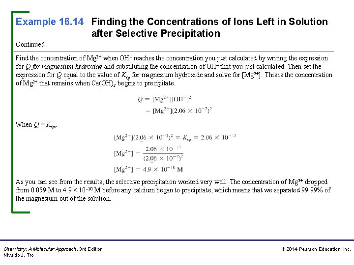
Example 16. 14 Finding the Concentrations of Ions Left in Solution after Selective Precipitation Continued Find the concentration of Mg 2+ when OH– reaches the concentration you just calculated by writing the expression for Q for magnesium hydroxide and substituting the concentration of OH– that you just calculated. Then set the expression for Q equal to the value of Ksp for magnesium hydroxide and solve for [Mg 2+]. This is the concentration of Mg 2+ that remains when Ca(OH)2 begins to precipitate. When Q = Ksp, As you can see from the results, the selective precipitation worked very well. The concentration of Mg 2+ dropped from 0. 059 M to 4. 9 × 10– 10 M before any calcium began to precipitate, which means that we separated 99. 99% of the magnesium out of the solution. Chemistry: A Molecular Approach, 3 rd Edition Nivaldo J. Tro © 2014 Pearson Education, Inc.

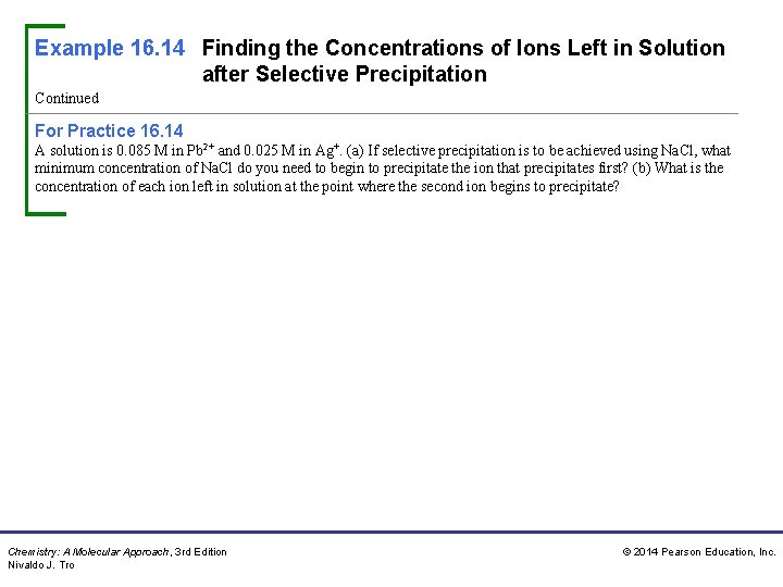
Example 16. 14 Finding the Concentrations of Ions Left in Solution after Selective Precipitation Continued For Practice 16. 14 A solution is 0. 085 M in Pb 2+ and 0. 025 M in Ag+. (a) If selective precipitation is to be achieved using Na. Cl, what minimum concentration of Na. Cl do you need to begin to precipitate the ion that precipitates first? (b) What is the concentration of each ion left in solution at the point where the second ion begins to precipitate? Chemistry: A Molecular Approach, 3 rd Edition Nivaldo J. Tro © 2014 Pearson Education, Inc.

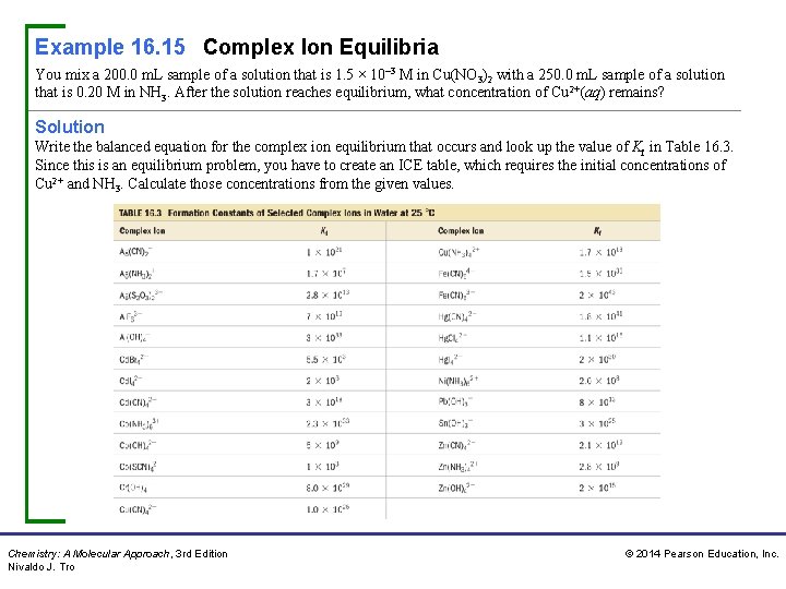
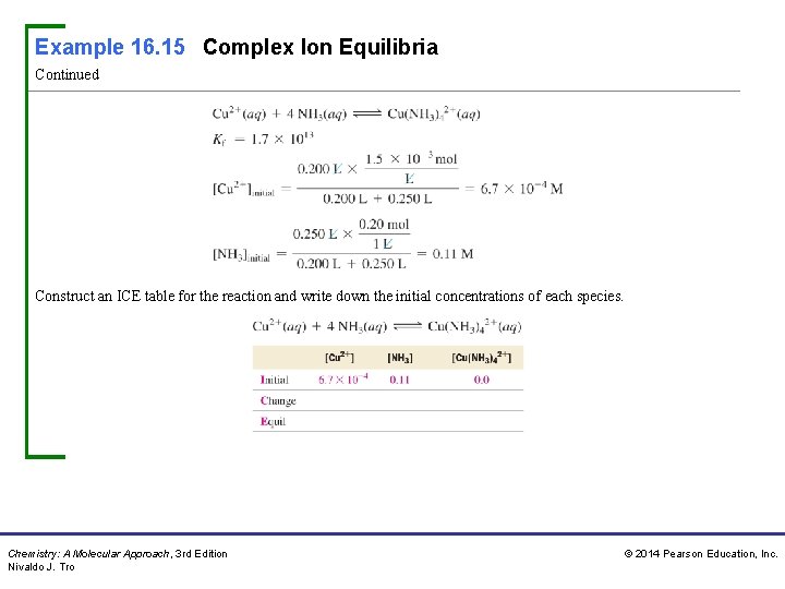
Example 16. 15 Complex Ion Equilibria You mix a 200. 0 m. L sample of a solution that is 1. 5 × 10– 3 M in Cu(NO 3)2 with a 250. 0 m. L sample of a solution that is 0. 20 M in NH 3. After the solution reaches equilibrium, what concentration of Cu 2+(aq) remains? Solution Write the balanced equation for the complex ion equilibrium that occurs and look up the value of Kf in Table 16. 3. Since this is an equilibrium problem, you have to create an ICE table, which requires the initial concentrations of Cu 2+ and NH 3. Calculate those concentrations from the given values. Chemistry: A Molecular Approach, 3 rd Edition Nivaldo J. Tro © 2014 Pearson Education, Inc.

Example 16. 15 Complex Ion Equilibria Continued Construct an ICE table for the reaction and write down the initial concentrations of each species. Chemistry: A Molecular Approach, 3 rd Edition Nivaldo J. Tro © 2014 Pearson Education, Inc.

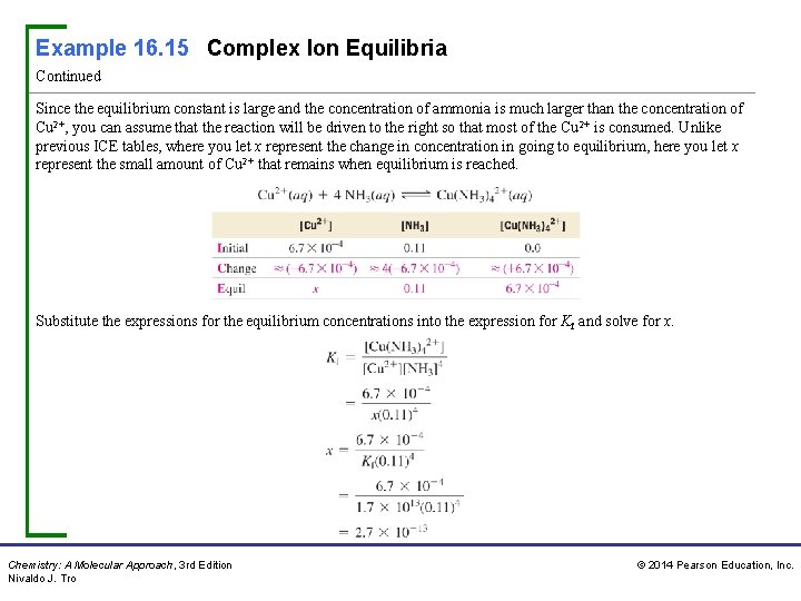
Example 16. 15 Complex Ion Equilibria Continued Since the equilibrium constant is large and the concentration of ammonia is much larger than the concentration of Cu 2+, you can assume that the reaction will be driven to the right so that most of the Cu 2+ is consumed. Unlike previous ICE tables, where you let x represent the change in concentration in going to equilibrium, here you let x represent the small amount of Cu 2+ that remains when equilibrium is reached. Substitute the expressions for the equilibrium concentrations into the expression for Kf and solve for x. Chemistry: A Molecular Approach, 3 rd Edition Nivaldo J. Tro © 2014 Pearson Education, Inc.

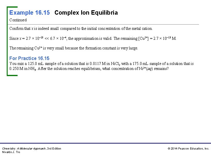
Example 16. 15 Complex Ion Equilibria Continued Confirm that x is indeed small compared to the initial concentration of the metal cation. Since x = 2. 7 × 10– 13 << 6. 7 × 10– 4, the approximation is valid. The remaining [Cu 2+] = 2. 7 × 10– 13 M. The remaining Cu 2+ is very small because the formation constant is very large. For Practice 16. 15 You mix a 125. 0 m. L sample of a solution that is 0. 0117 M in Ni. Cl 2 with a 175. 0 m. L sample of a solution that is 0. 250 M in NH 3. After the solution reaches equilibrium, what concentration of Ni 2+(aq) remains? Chemistry: A Molecular Approach, 3 rd Edition Nivaldo J. Tro © 2014 Pearson Education, Inc.