Dynamic Programming Divide and Conquer and Greedy Algorithms

Dynamic Programming Divide and Conquer and Greedy Algorithms are powerful techniques in situations which fit their strengths l Dynamic Programming can usually be used in a broader set of applications l – DP uses some graph algorithm techniques in a specific fashion l Some call Dynamic Programming and Linear Programming (next chapter) the "Sledgehammers" of algorithmic tools – "Programming" in these names does not come from writing code as we normally consider it – These names were given before modern computers and programming was tied to the meaning of "planning" CS 312 – Dynamic Programming 1

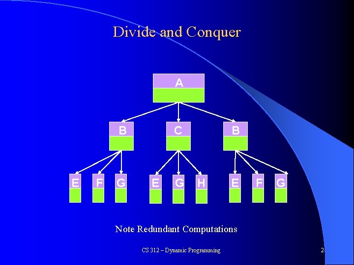
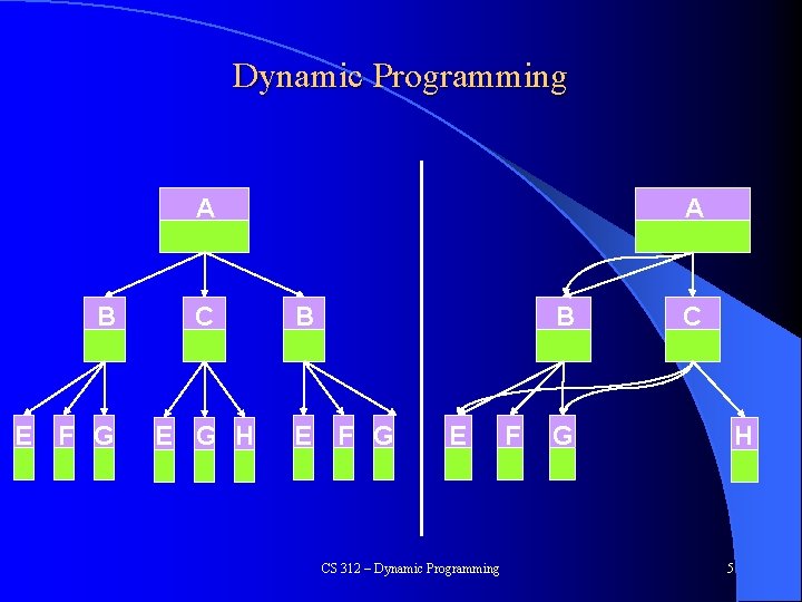
Divide and Conquer A B E F G C E G B H E F G Note Redundant Computations CS 312 – Dynamic Programming 2

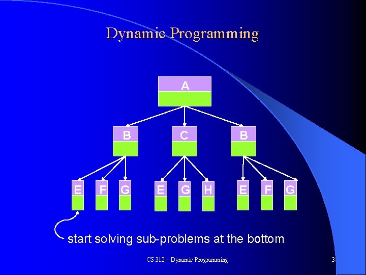
Dynamic Programming A B E F G C E G B H E F G start solving sub-problems at the bottom CS 312 – Dynamic Programming 3

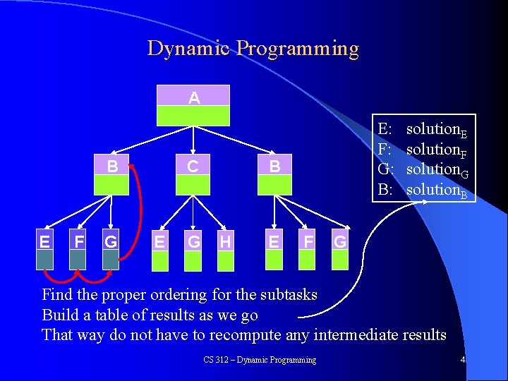
Dynamic Programming A B E F G C E G E: F: G: B: B H E F solution. E solution. F solution. G solution. B G Find the proper ordering for the subtasks Build a table of results as we go That way do not have to recompute any intermediate results CS 312 – Dynamic Programming 4

Dynamic Programming A B E F G C E G H A B B E F G E CS 312 – Dynamic Programming F C H G 5

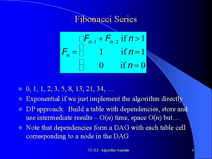
Fibonacci Series 0, 1, 1, 2, 3, 5, 8, 13, 21, 34, … l Exponential if we just implement the algorithm directly l DP approach: Build a table with dependencies, store and use intermediate results – O(n) time, space O(n) but… l Note that dependencies form a DAG with each table cell corresponding to a node in the DAG l CS 312 - Algorithm Analysis 6

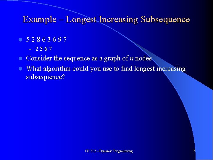
Example – Longest Increasing Subsequence l 52863697 – 2367 Consider the sequence as a graph of n nodes l What algorithm could you use to find longest increasing subsequence? l CS 312 – Dynamic Programming 7

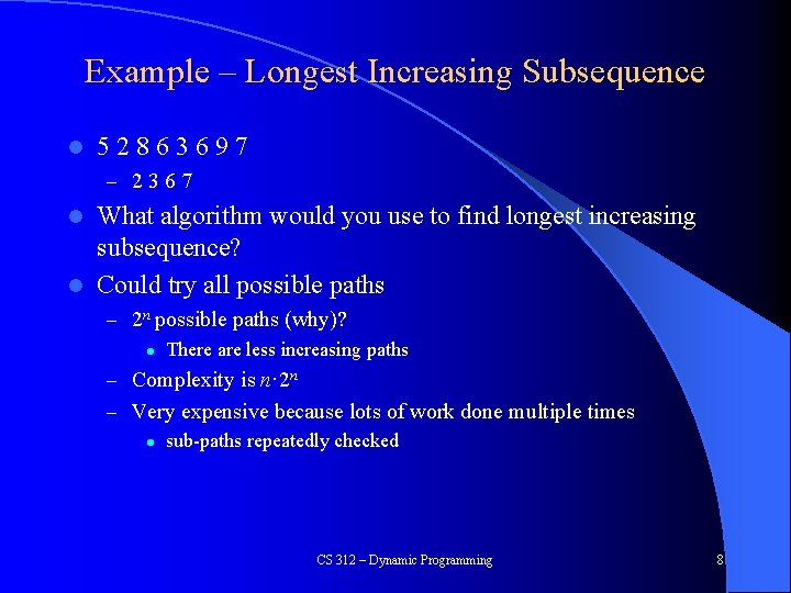
Example – Longest Increasing Subsequence l 52863697 – 2367 What algorithm would you use to find longest increasing subsequence? l Could try all possible paths l – 2 n possible paths (why)? l There are less increasing paths – Complexity is n· 2 n – Very expensive because lots of work done multiple times l sub-paths repeatedly checked CS 312 – Dynamic Programming 8

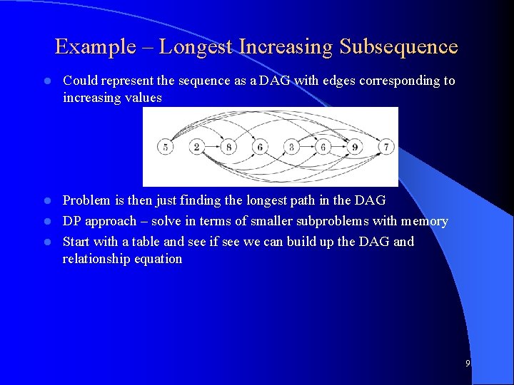
Example – Longest Increasing Subsequence l Could represent the sequence as a DAG with edges corresponding to increasing values Problem is then just finding the longest path in the DAG l DP approach – solve in terms of smaller subproblems with memory l Start with a table and see if see we can build up the DAG and relationship equation l 9

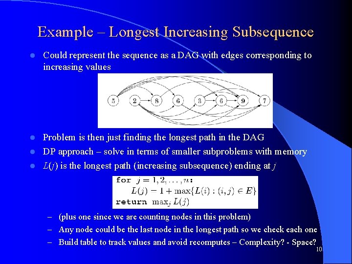
Example – Longest Increasing Subsequence l Could represent the sequence as a DAG with edges corresponding to increasing values Problem is then just finding the longest path in the DAG l DP approach – solve in terms of smaller subproblems with memory l L(j) is the longest path (increasing subsequence) ending at j l – (plus one since we are counting nodes in this problem) – Any node could be the last node in the longest path so we check each one – Build table to track values and avoid recomputes – Complexity? - Space? 10

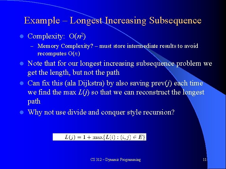
Example – Longest Increasing Subsequence l Complexity: O(n 2) – Memory Complexity? – must store intermediate results to avoid recomputes O(n) Note that for our longest increasing subsequence problem we get the length, but not the path l Can fix this (ala Dijkstra) by also saving prev(j) each time we find the max L(j) so that we can reconstruct the longest path l Why not use divide and conquer style recursion? l CS 312 – Dynamic Programming 11

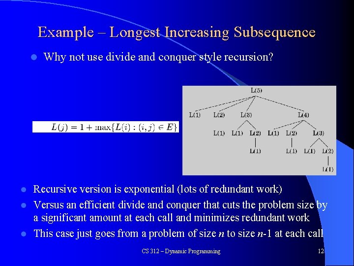
Example – Longest Increasing Subsequence l Why not use divide and conquer style recursion? Recursive version is exponential (lots of redundant work) l Versus an efficient divide and conquer that cuts the problem size by a significant amount at each call and minimizes redundant work l This case just goes from a problem of size n to size n-1 at each call l CS 312 – Dynamic Programming 12

When is Dynamic Programming Efficient Anytime we have a collection of subproblems such that: l There is an ordering on the subproblems, and a relation that shows how to solve a subproblem given the answers to "smaller" subproblems, that is, subproblems that appear earlier in the ordering – No cycles! l Problem becomes an implicit DAG with each subproblem represented by a node, with edges giving dependencies l – Just one order to solve it? - Any linearization works CS 312 – Dynamic Programming 13

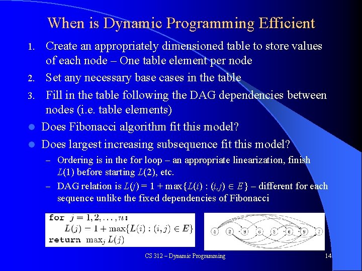
When is Dynamic Programming Efficient 1. 2. 3. l l Create an appropriately dimensioned table to store values of each node – One table element per node Set any necessary base cases in the table Fill in the table following the DAG dependencies between nodes (i. e. table elements) Does Fibonacci algorithm fit this model? Does largest increasing subsequence fit this model? – Ordering is in the for loop – an appropriate linearization, finish L(1) before starting L(2), etc. – DAG relation is L(j) = 1 + max{L(i) : (i, j) E} – different for each sequence unlike the fixed dependencies of Fibonacci CS 312 – Dynamic Programming 14

When is Dynamic Programming Optimal? l DP is optimal when the optimality property is met – First make sure solution is correct The optimality property: An optimal solution to a problem is built from optimal solutions to sub-problems l Question to consider: Can we divide the problem into subproblems such that the optimal solutions to each of the subproblems combine into an optimal solution for the entire problem? l CS 312 – Dynamic Programming 15

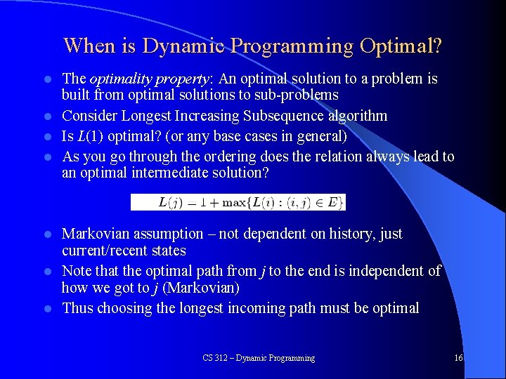
When is Dynamic Programming Optimal? The optimality property: An optimal solution to a problem is built from optimal solutions to sub-problems l Consider Longest Increasing Subsequence algorithm l Is L(1) optimal? (or any base cases in general) l As you go through the ordering does the relation always lead to an optimal intermediate solution? l Markovian assumption – not dependent on history, just current/recent states l Note that the optimal path from j to the end is independent of how we got to j (Markovian) l Thus choosing the longest incoming path must be optimal l CS 312 – Dynamic Programming 16

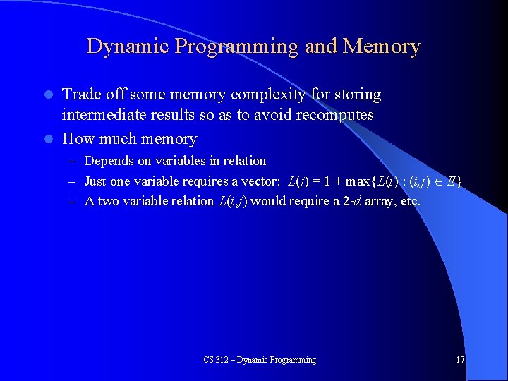
Dynamic Programming and Memory Trade off some memory complexity for storing intermediate results so as to avoid recomputes l How much memory l – Depends on variables in relation – Just one variable requires a vector: L(j) = 1 + max{L(i) : (i, j) E} – A two variable relation L(i, j) would require a 2 -d array, etc. CS 312 – Dynamic Programming 17

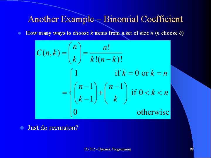
Another Example – Binomial Coefficient l l How many ways to choose k items from a set of size n (n choose k) Just do recursion? CS 312 – Dynamic Programming 18

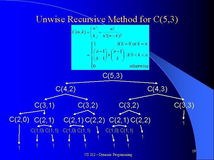
Unwise Recursive Method for C(5, 3) C(4, 2) C(3, 1) C(2, 0) C(2, 1) C(4, 3) C(3, 2) C(2, 1) C(2, 2) C(1, 0) C(1, 1) 1 1 1 C(3, 3) 1 1 CS 312 – Dynamic Programming 19

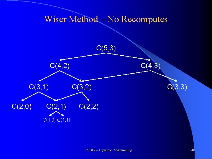
Wiser Method – No Recomputes C(5, 3) C(4, 2) C(3, 1) C(2, 0) C(2, 1) C(4, 3) C(3, 2) C(3, 3) C(2, 2) C(1, 0) C(1, 1) CS 312 – Dynamic Programming 20

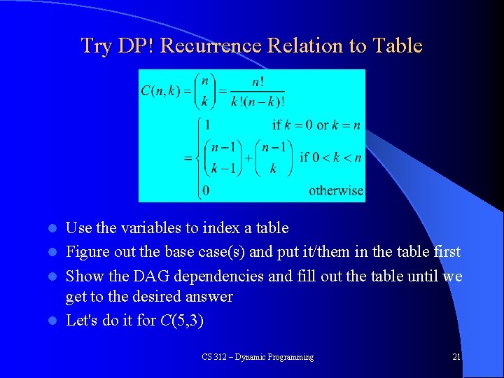
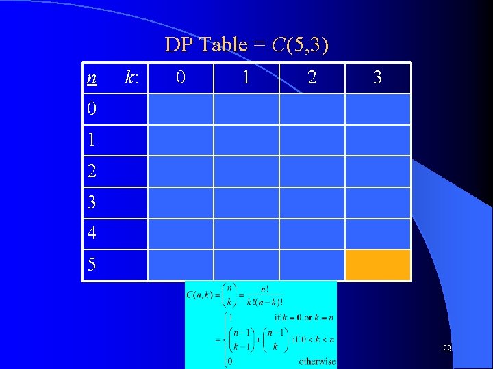
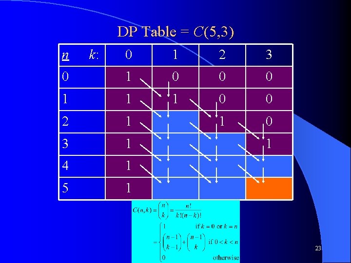
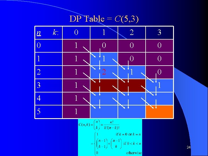
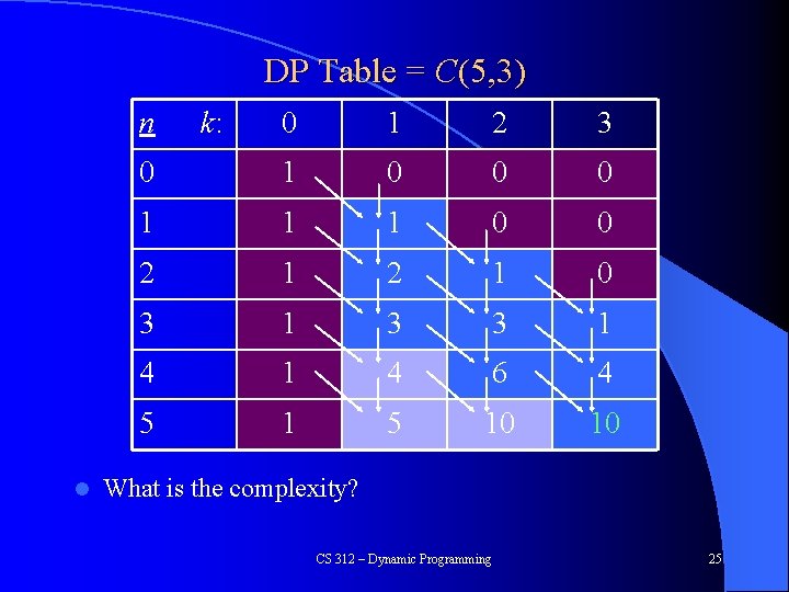
Try DP! Recurrence Relation to Table Use the variables to index a table l Figure out the base case(s) and put it/them in the table first l Show the DAG dependencies and fill out the table until we get to the desired answer l Let's do it for C(5, 3) l CS 312 – Dynamic Programming 21

DP Table = C(5, 3) n k: 0 1 2 3 4 5 CS 312 – Dynamic Programming 22

DP Table = C(5, 3) n k: 0 1 2 3 0 1 0 0 0 1 1 1 0 0 2 1 1 0 3 1 4 1 5 1 1 CS 312 – Dynamic Programming 23

DP Table = C(5, 3) n k: 0 1 2 3 0 1 0 0 0 1 1 1 0 0 2 1 0 3 1 4 1 5 1 1 CS 312 – Dynamic Programming 24

DP Table = C(5, 3) n l k: 0 1 2 3 0 1 0 0 0 1 1 1 0 0 2 1 0 3 1 3 3 1 4 6 4 5 10 10 What is the complexity? CS 312 – Dynamic Programming 25

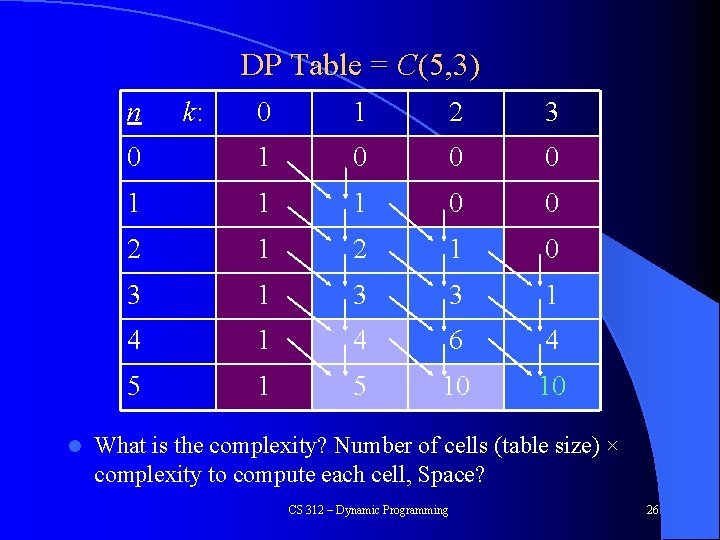
DP Table = C(5, 3) n l k: 0 1 2 3 0 1 0 0 0 1 1 1 0 0 2 1 0 3 1 3 3 1 4 6 4 5 10 10 What is the complexity? Number of cells (table size) × complexity to compute each cell, Space? CS 312 – Dynamic Programming 26

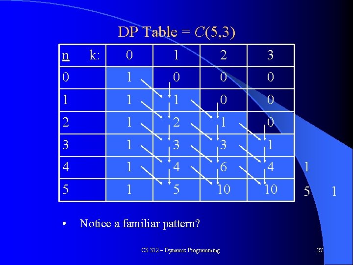
DP Table = C(5, 3) n 0 1 2 3 0 1 0 0 0 1 1 1 0 0 2 1 0 3 1 3 3 1 4 6 4 1 5 10 10 5 • k: 1 Notice a familiar pattern? CS 312 – Dynamic Programming 27

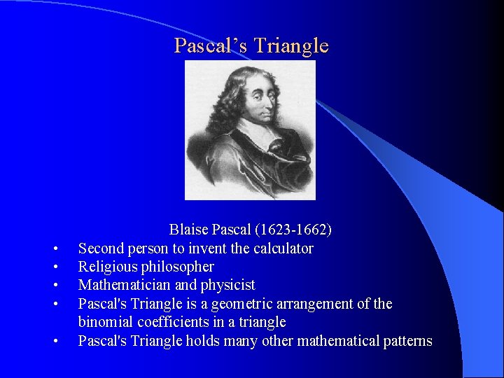
Pascal’s Triangle • • • Blaise Pascal (1623 -1662) Second person to invent the calculator Religious philosopher Mathematician and physicist Pascal's Triangle is a geometric arrangement of the binomial coefficients in a triangle Pascal's Triangle holds many other mathematical patterns

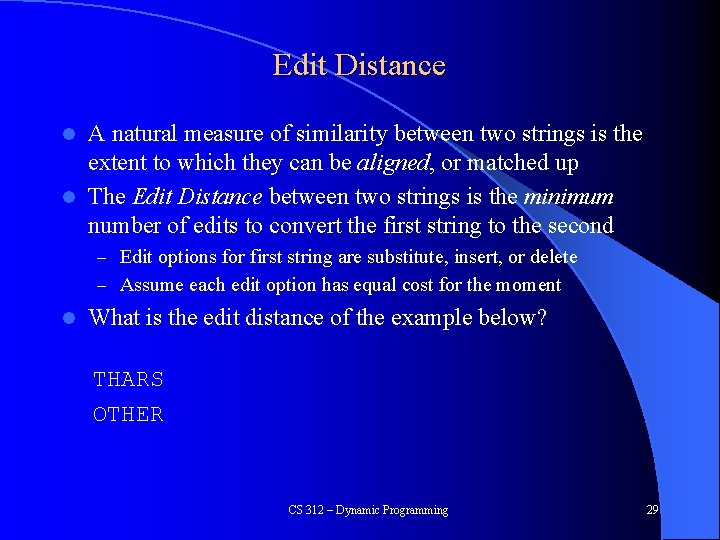
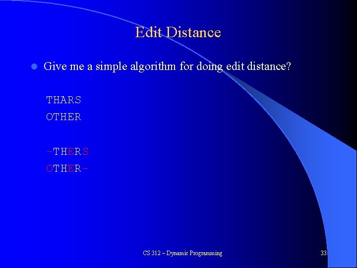
Edit Distance A natural measure of similarity between two strings is the extent to which they can be aligned, or matched up l The Edit Distance between two strings is the minimum number of edits to convert the first string to the second l – Edit options for first string are substitute, insert, or delete – Assume each edit option has equal cost for the moment l What is the edit distance of the example below? THARS OTHER CS 312 – Dynamic Programming 29

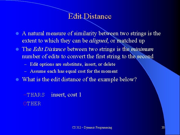
Edit Distance A natural measure of similarity between two strings is the extent to which they can be aligned, or matched up l The Edit Distance between two strings is the minimum number of edits to convert the first string to the second l – Edit options are substitute, insert, or delete – Assume each has equal cost for the moment l What is the edit distance of the example below? -THARS OTHER insert, cost 1 CS 312 – Dynamic Programming 30

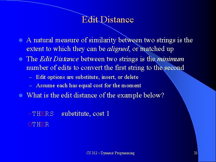
Edit Distance A natural measure of similarity between two strings is the extent to which they can be aligned, or matched up l The Edit Distance between two strings is the minimum number of edits to convert the first string to the second l – Edit options are substitute, insert, or delete – Assume each has equal cost for the moment l What is the edit distance of the example below? -THERS OTHER substitute, cost 1 CS 312 – Dynamic Programming 31

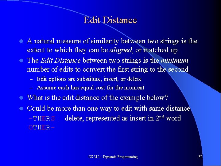
Edit Distance A natural measure of similarity between two strings is the extent to which they can be aligned, or matched up l The Edit Distance between two strings is the minimum number of edits to convert the first string to the second l – Edit options are substitute, insert, or delete – Assume each has equal cost for the moment What is the edit distance of the example below? l Could be more than one way to edit with same distance -THERS delete, represented as insert in 2 nd word OTHERl CS 312 – Dynamic Programming 32

Edit Distance l Give me a simple algorithm for doing edit distance? THARS OTHER -THERS OTHER- CS 312 – Dynamic Programming 33

Edit Distance l l l 1. 2. Give me a simple algorithm for doing edit distance? Number of possible alignments grows exponentially with string length n, so we try DP to solve it efficiently Two things to consider Is there an ordering on the subproblems, and a relation that shows how to solve a subproblem given the answers to "smaller" subproblems, that is, subproblems that appear earlier in the ordering Is it the case that an optimal solution to a problem is built from optimal solutions to sub-problems CS 312 – Dynamic Programming 34

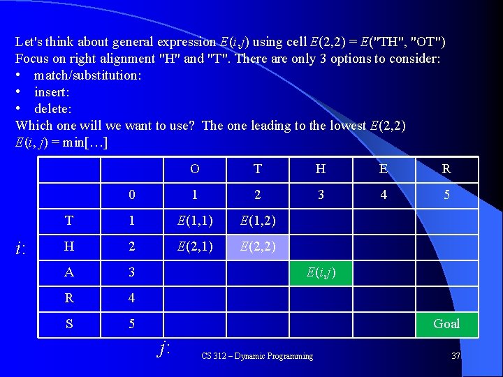
DP approach to Edit Distance l l l Assume two strings x and y of length m and n respectively Consider the edit subproblem E(i, j) = E(x[1…i], y[1…j]) For x = "taco" and y = "texco" E(2, 3) = E("ta", "tex") The final solution is E(m, n) = E(4, 5) This notation gives a natural way to start from small cases and build up to larger ones – l Common paradigm for breaking down DP problems Let's start by building a table – – What are the base cases? What is the relationship E(i, j) of the next open cell based on previous cells? CS 312 – Dynamic Programming 35

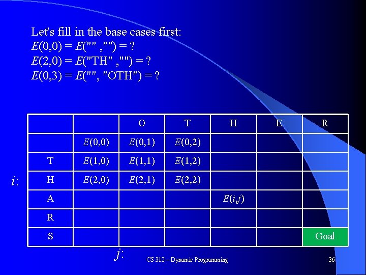
Let's fill in the base cases first: E(0, 0) = E("" , "") = ? E(2, 0) = E("TH" , "") = ? E(0, 3) = E("", "OTH") = ? i: O T E(0, 0) E(0, 1) E(0, 2) T E(1, 0) E(1, 1) E(1, 2) H E(2, 0) E(2, 1) E(2, 2) A H E R E(i, j) R S Goal j: CS 312 – Dynamic Programming 36

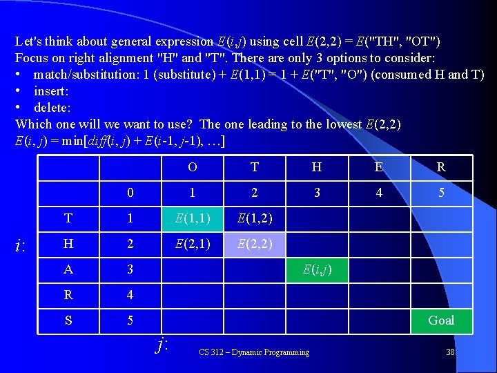
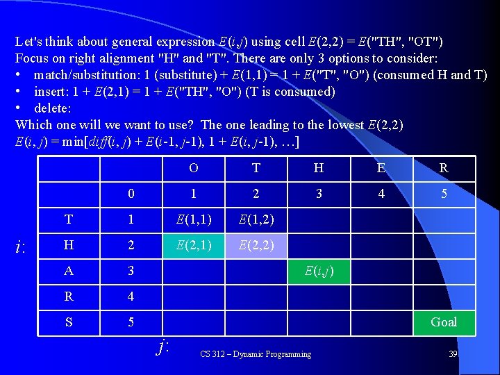
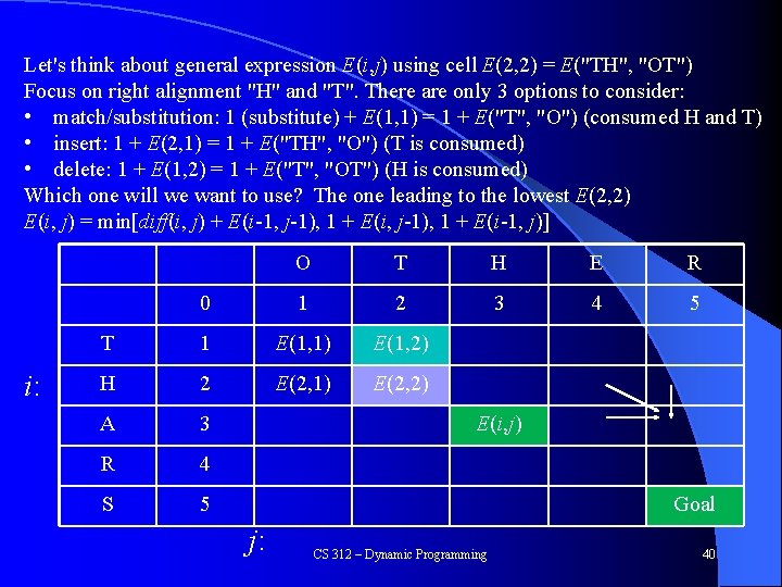
Let's think about general expression E(i, j) using cell E(2, 2) = E("TH", "OT") Focus on right alignment "H" and "T". There are only 3 options to consider: • match/substitution: • insert: • delete: Which one will we want to use? The one leading to the lowest E(2, 2) E(i, j) = min[…] i: O T H E R 0 1 2 3 4 5 T 1 E(1, 1) E(1, 2) H 2 E(2, 1) E(2, 2) A 3 R 4 S 5 E(i, j) Goal j: CS 312 – Dynamic Programming 37

Let's think about general expression E(i, j) using cell E(2, 2) = E("TH", "OT") Focus on right alignment "H" and "T". There are only 3 options to consider: • match/substitution: 1 (substitute) + E(1, 1) = 1 + E("T", "O") (consumed H and T) • insert: • delete: Which one will we want to use? The one leading to the lowest E(2, 2) E(i, j) = min[diff(i, j) + E(i-1, j-1), …] i: O T H E R 0 1 2 3 4 5 T 1 E(1, 1) E(1, 2) H 2 E(2, 1) E(2, 2) A 3 R 4 S 5 E(i, j) Goal j: CS 312 – Dynamic Programming 38

Let's think about general expression E(i, j) using cell E(2, 2) = E("TH", "OT") Focus on right alignment "H" and "T". There are only 3 options to consider: • match/substitution: 1 (substitute) + E(1, 1) = 1 + E("T", "O") (consumed H and T) • insert: 1 + E(2, 1) = 1 + E("TH", "O") (T is consumed) • delete: Which one will we want to use? The one leading to the lowest E(2, 2) E(i, j) = min[diff(i, j) + E(i-1, j-1), 1 + E(i, j-1), …] i: O T H E R 0 1 2 3 4 5 T 1 E(1, 1) E(1, 2) H 2 E(2, 1) E(2, 2) A 3 R 4 S 5 E(i, j) Goal j: CS 312 – Dynamic Programming 39

Let's think about general expression E(i, j) using cell E(2, 2) = E("TH", "OT") Focus on right alignment "H" and "T". There are only 3 options to consider: • match/substitution: 1 (substitute) + E(1, 1) = 1 + E("T", "O") (consumed H and T) • insert: 1 + E(2, 1) = 1 + E("TH", "O") (T is consumed) • delete: 1 + E(1, 2) = 1 + E("T", "OT") (H is consumed) Which one will we want to use? The one leading to the lowest E(2, 2) E(i, j) = min[diff(i, j) + E(i-1, j-1), 1 + E(i-1, j)] i: O T H E R 0 1 2 3 4 5 T 1 E(1, 1) E(1, 2) H 2 E(2, 1) E(2, 2) A 3 R 4 S 5 E(i, j) Goal j: CS 312 – Dynamic Programming 40

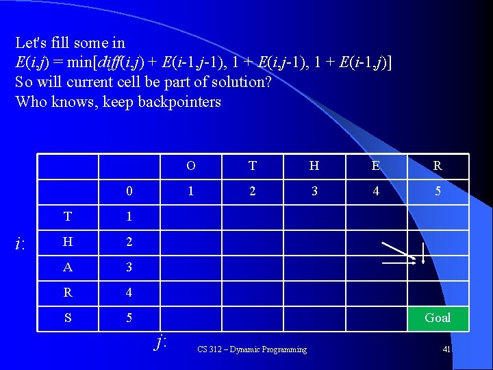
Let's fill some in E(i, j) = min[diff(i, j) + E(i-1, j-1), 1 + E(i-1, j)] So will current cell be part of solution? Who knows, keep backpointers 0 i: T 1 H 2 A 3 R 4 S 5 O T H E R 1 2 3 4 5 Goal j: CS 312 – Dynamic Programming 41

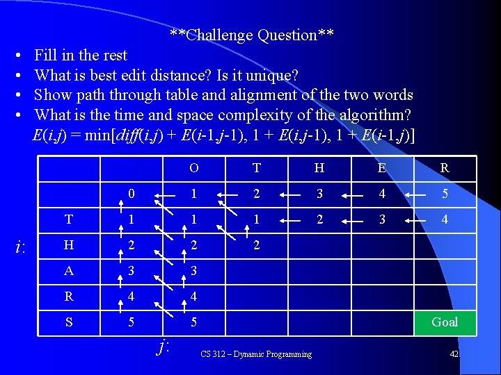
**Challenge Question** • • i: Fill in the rest What is best edit distance? Is it unique? Show path through table and alignment of the two words What is the time and space complexity of the algorithm? E(i, j) = min[diff(i, j) + E(i-1, j-1), 1 + E(i-1, j)] O T H E R 0 1 2 3 4 5 T 1 1 1 2 3 4 H 2 2 2 A 3 3 R 4 4 S 5 5 j: Goal CS 312 – Dynamic Programming 42

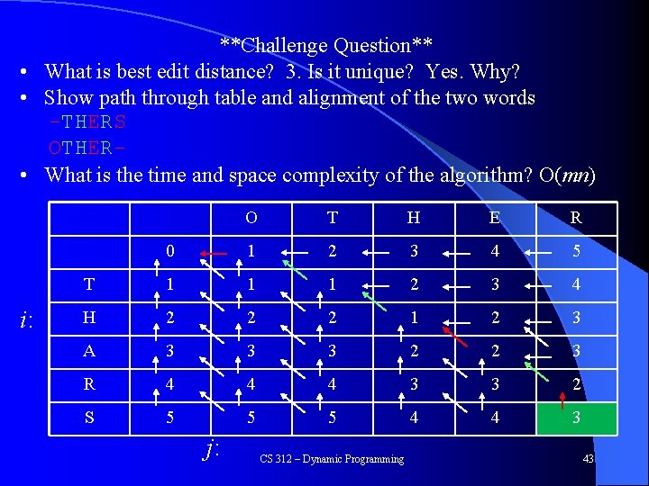
**Challenge Question** • What is best edit distance? 3. Is it unique? Yes. Why? • Show path through table and alignment of the two words -THERS OTHER • What is the time and space complexity of the algorithm? O(mn) i: O T H E R 0 1 2 3 4 5 T 1 1 1 2 3 4 H 2 2 2 1 2 3 A 3 3 3 2 2 3 R 4 4 4 3 3 2 S 5 5 5 4 4 3 j: CS 312 – Dynamic Programming 43

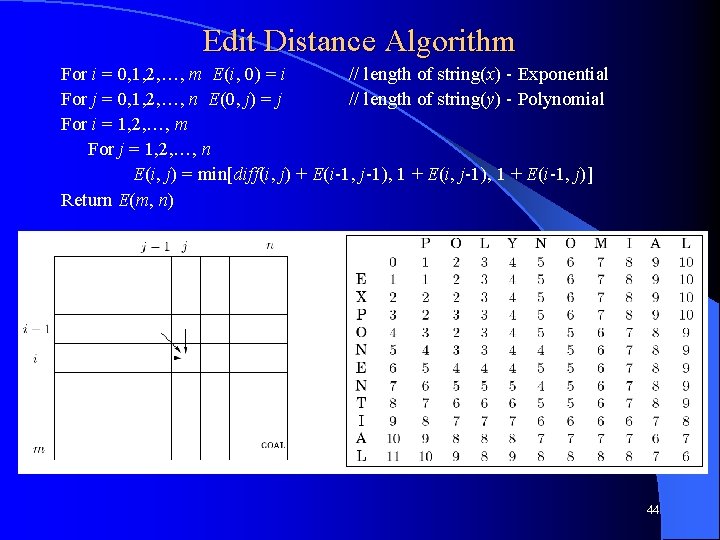
Edit Distance Algorithm For i = 0, 1, 2, …, m E(i, 0) = i // length of string(x) - Exponential For j = 0, 1, 2, …, n E(0, j) = j // length of string(y) - Polynomial For i = 1, 2, …, m For j = 1, 2, …, n E(i, j) = min[diff(i, j) + E(i-1, j-1), 1 + E(i-1, j)] Return E(m, n) 44

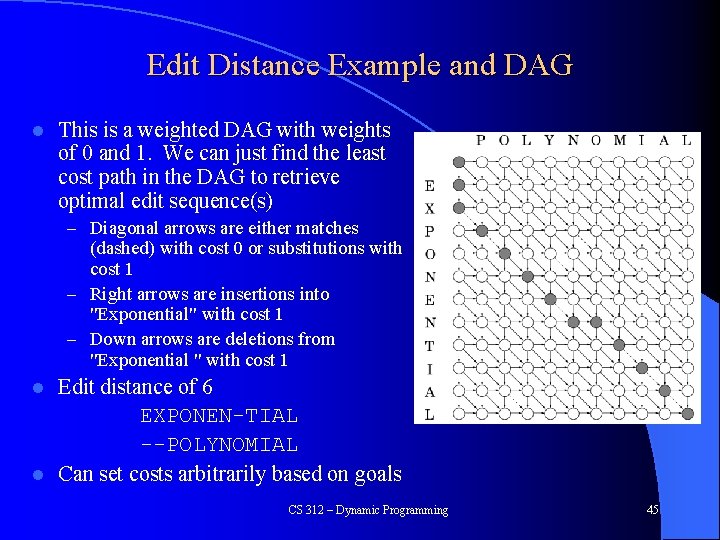
Edit Distance Example and DAG l This is a weighted DAG with weights of 0 and 1. We can just find the least cost path in the DAG to retrieve optimal edit sequence(s) – Diagonal arrows are either matches (dashed) with cost 0 or substitutions with cost 1 – Right arrows are insertions into "Exponential" with cost 1 – Down arrows are deletions from "Exponential " with cost 1 Edit distance of 6 EXPONEN-TIAL --POLYNOMIAL l Can set costs arbitrarily based on goals l CS 312 – Dynamic Programming 45

Space Requirements l l l Basic table is m × n which is O(n 2) assuming m and n are similar What order options can we use to calculate cells But do we really need to use O(n 2) memory? How can we implement edit-distance using only O(n) memory? However, What about prev pointers and extracting the actual alignment with the O(n) approach? – Thus, in practice space is O(n 2) CS 312 – Dynamic Programming 46

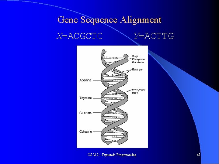
Gene Sequence Alignment X=ACGCTC Y=ACTTG CS 312 – Dynamic Programming 47

Needleman-Wunsch Algorithm l Gene Sequence Alignment a type of Edit Distance ACGCT-C A--CTTG – Uses Needleman-Wunsch Algorithm – This is just edit distance with a different edge weighting (i. e. different edge lengths on DAG and we find shortest path) – You will use Needleman-Wunsch in your project l Cost (Typical Needleman-Wunsch costs are shown): – – l Match: cmatch = -3 (a reward) Insertion into x (= deletion from y): cindel = 5 Insertion into y (= deletion from x): cindel = 5 Substitutions of a character from x into y (or from y into x): csub = 1 You will use the above costs in your HW and project – Does that change the base cases? CS 312 – Dynamic Programming 48

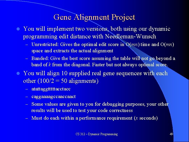
Gene Alignment Project l You will implement two versions, both using our dynamic programming edit distance with Needleman-Wunsch – Unrestricted: Gives the optimal edit score in O(mn) time and O(mn) space and extracts the actual alignment – Banded: Give the best score assuming the table will not go beyond a band of k from the diagonal. Faster but not always optimal score. l You will align 10 supplied real gene sequences with each other (100/2 = 50 alignments) – atattaggtttttacc – caggaaaagccaact – Some values are given to you for debugging purposes, your other results will be used to test your code correctness – Must do each within a performance requirement (x seconds) CS 312 – Dynamic Programming 49

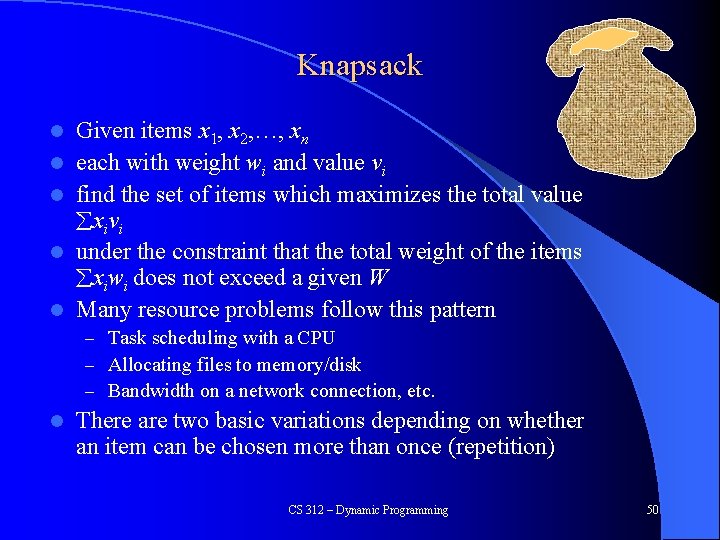
Knapsack l l l Given items x 1, x 2, …, xn each with weight wi and value vi find the set of items which maximizes the total value xivi under the constraint that the total weight of the items xiwi does not exceed a given W Many resource problems follow this pattern – Task scheduling with a CPU – Allocating files to memory/disk – Bandwidth on a network connection, etc. l There are two basic variations depending on whether an item can be chosen more than once (repetition) CS 312 – Dynamic Programming 50

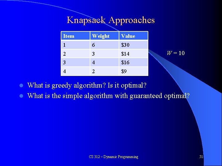
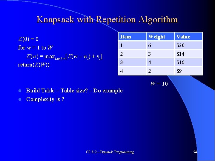
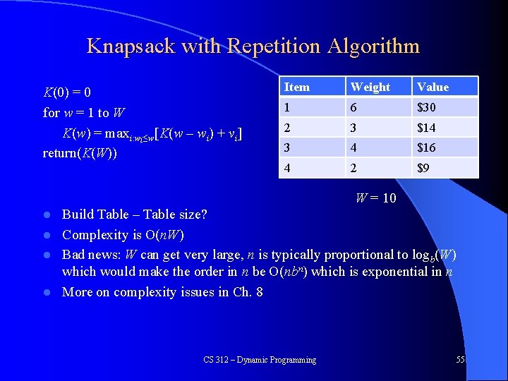
Knapsack Approaches Item Weight Value 1 6 $30 2 3 $14 3 4 $16 4 2 $9 W = 10 What is greedy algorithm? Is it optimal? l What is the simple algorithm with guaranteed optimal? l CS 312 – Dynamic Programming 51

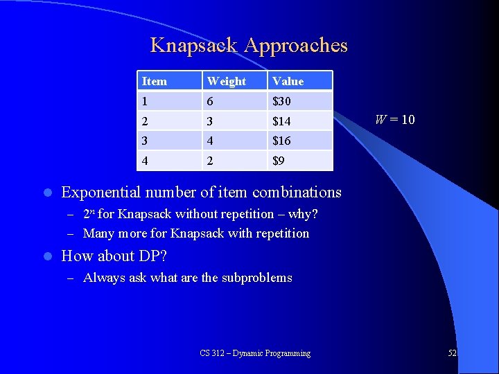
Knapsack Approaches l Item Weight Value 1 6 $30 2 3 $14 3 4 $16 4 2 $9 W = 10 Exponential number of item combinations – 2 n for Knapsack without repetition – why? – Many more for Knapsack with repetition l How about DP? – Always ask what are the subproblems CS 312 – Dynamic Programming 52

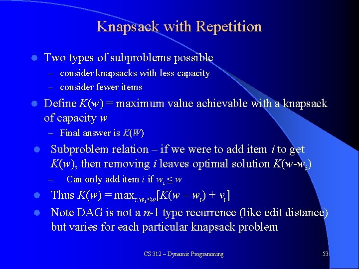
Knapsack with Repetition l Two types of subproblems possible – consider knapsacks with less capacity – consider fewer items l Define K(w) = maximum value achievable with a knapsack of capacity w – Final answer is K(W) l Subproblem relation – if we were to add item i to get K(w), then removing i leaves optimal solution K(w-wi) – Can only add item i if wi ≤ w Thus K(w) = maxi: wi≤w[K(w – wi) + vi] l Note DAG is not a n-1 type recurrence (like edit distance) but varies for each particular knapsack problem l CS 312 – Dynamic Programming 53

Knapsack with Repetition Algorithm K(0) = 0 for w = 1 to W K(w) = maxi: wi≤w[K(w – wi) + vi] return(K(W)) Item Weight Value 1 6 $30 2 3 $14 3 4 $16 4 2 $9 W = 10 Build Table – Table size? – Do example l Complexity is ? l CS 312 – Dynamic Programming 54

Knapsack with Repetition Algorithm K(0) = 0 for w = 1 to W K(w) = maxi: wi≤w[K(w – wi) + vi] return(K(W)) Item Weight Value 1 6 $30 2 3 $14 3 4 $16 4 2 $9 W = 10 Build Table – Table size? l Complexity is O(n. W) l Bad news: W can get very large, n is typically proportional to logb(W) which would make the order in n be O(nbn) which is exponential in n l More on complexity issues in Ch. 8 l CS 312 – Dynamic Programming 55

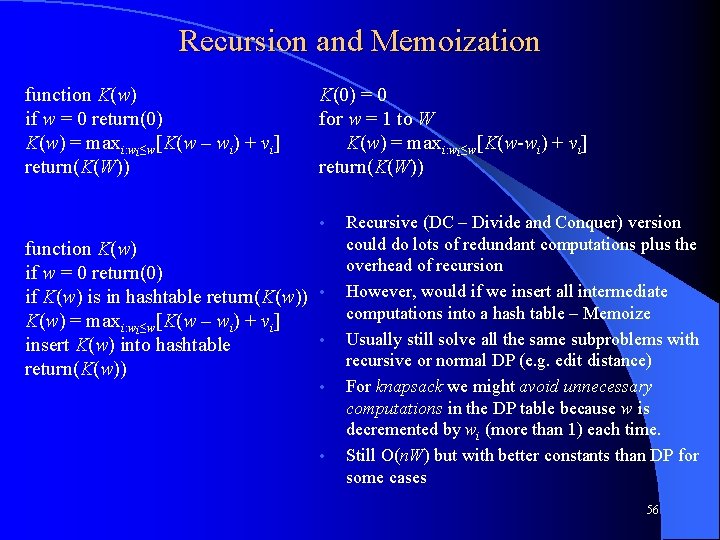
Recursion and Memoization function K(w) if w = 0 return(0) K(w) = maxi: wi≤w[K(w – wi) + vi] return(K(W)) K(0) = 0 for w = 1 to W K(w) = maxi: wi≤w[K(w-wi) + vi] return(K(W)) • function K(w) if w = 0 return(0) if K(w) is in hashtable return(K(w)) K(w) = maxi: wi≤w[K(w – wi) + vi] insert K(w) into hashtable return(K(w)) • • Recursive (DC – Divide and Conquer) version could do lots of redundant computations plus the overhead of recursion However, would if we insert all intermediate computations into a hash table – Memoize Usually still solve all the same subproblems with recursive or normal DP (e. g. edit distance) For knapsack we might avoid unnecessary computations in the DP table because w is decremented by wi (more than 1) each time. Still O(n. W) but with better constants than DP for some cases 56

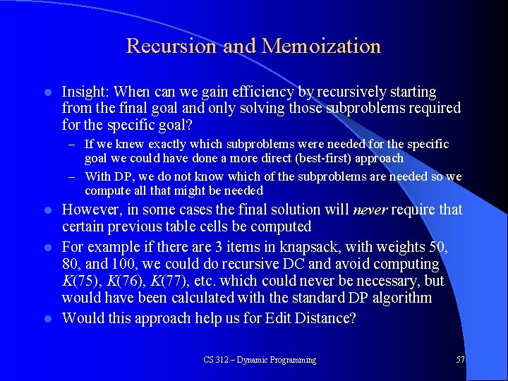
Recursion and Memoization l Insight: When can we gain efficiency by recursively starting from the final goal and only solving those subproblems required for the specific goal? – If we knew exactly which subproblems were needed for the specific goal we could have done a more direct (best-first) approach – With DP, we do not know which of the subproblems are needed so we compute all that might be needed However, in some cases the final solution will never require that certain previous table cells be computed l For example if there are 3 items in knapsack, with weights 50, 80, and 100, we could do recursive DC and avoid computing K(75), K(76), K(77), etc. which could never be necessary, but would have been calculated with the standard DP algorithm l Would this approach help us for Edit Distance? l CS 312 – Dynamic Programming 57

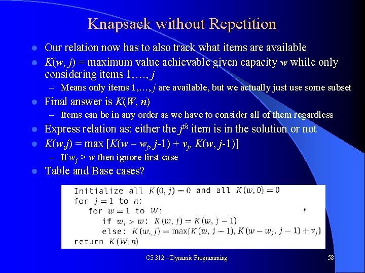
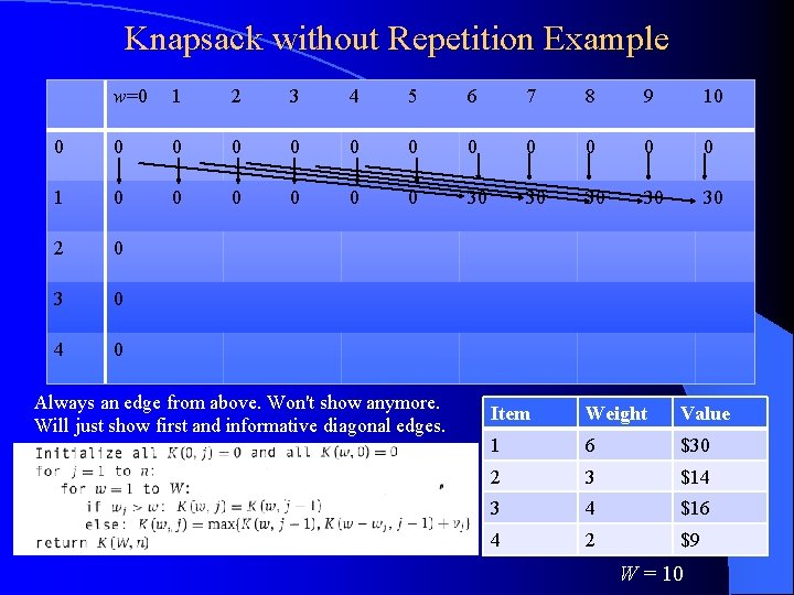
Knapsack without Repetition Our relation now has to also track what items are available l K(w, j) = maximum value achievable given capacity w while only considering items 1, …, j l – Means only items 1, …, j are available, but we actually just use some subset l Final answer is K(W, n) – Items can be in any order as we have to consider all of them regardless Express relation as: either the jth item is in the solution or not l K(w, j) = max [K(w – wj, j-1) + vj, K(w, j-1)] l – If wj > w then ignore first case l Table and Base cases? CS 312 – Dynamic Programming 58

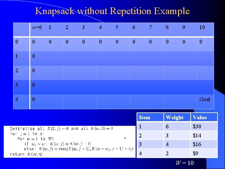
Knapsack without Repetition Example w=0 1 2 3 4 5 6 7 8 9 10 0 0 0 1 0 2 0 3 0 4 0 Goal Item Weight Value 1 6 $30 2 3 $14 3 4 $16 4 2 $9 W = 10

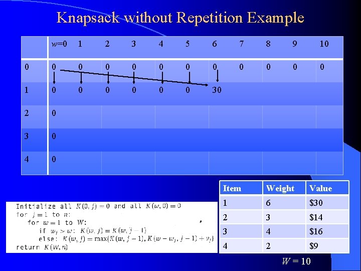
Knapsack without Repetition Example w=0 1 2 3 4 5 6 7 8 9 10 0 0 0 1 0 0 0 30 2 0 3 0 4 0 Item Weight Value 1 6 $30 2 3 $14 3 4 $16 4 2 $9 W = 10

Knapsack without Repetition Example w=0 1 2 3 4 5 6 7 8 9 10 0 0 0 1 0 0 0 30 30 30 2 0 3 0 4 0 Always an edge from above. Won't show anymore. Will just show first and informative diagonal edges. Item Weight Value 1 6 $30 2 3 $14 3 4 $16 4 2 $9 W = 10

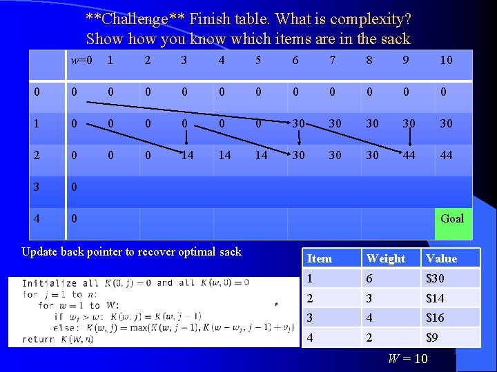
**Challenge** Finish table. What is complexity? Show you know which items are in the sack w=0 1 2 3 4 5 6 7 8 9 10 0 0 0 1 0 0 0 30 30 30 2 0 0 0 14 14 14 30 30 30 44 44 3 0 4 0 Update back pointer to recover optimal sack Goal Item Weight Value 1 6 $30 2 3 $14 3 4 $16 4 2 $9 W = 10

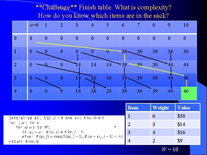
**Challenge** Finish table. What is complexity? How do you know which items are in the sack? w=0 1 2 3 4 5 6 7 8 9 10 0 0 0 1 0 0 0 30 30 30 2 0 0 0 14 14 14 30 30 30 44 44 3 0 0 0 14 16 16 30 30 30 44 46 4 0 0 9 14 16 23 30 30 39 44 46 Item Weight Value 1 6 $30 2 3 $14 3 4 $16 4 2 $9 W = 10

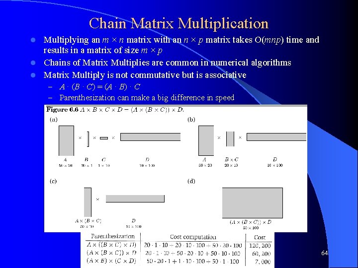
Chain Matrix Multiplication Multiplying an m × n matrix with an n × p matrix takes O(mnp) time and results in a matrix of size m × p l Chains of Matrix Multiplies are common in numerical algorithms l Matrix Multiply is not commutative but is associative l – A · (B · C) = (A · B) · C – Parenthesization can make a big difference in speed CS 312 – Dynamic Programming 64

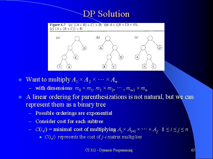
DP Solution l Want to multiply A 1 × A 2 × ··· × An – with dimensions m 0 × m 1, m 1 × m 2, ··· , mn-1 × mn l A linear ordering for parenthesizations is not natural, but we can represent them as a binary tree – Possible orderings are exponential – Consider cost for each subtree – C(i, j) = minimal cost of multiplying Ai × Ai+1 × ··· × Aj 1 ≤ i ≤ j ≤ n l C(i, j) represents the cost of j-i matrix multiplies CS 312 – Dynamic Programming 65

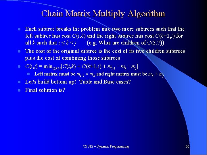
Chain Matrix Multiply Algorithm Each subtree breaks the problem into two more subtrees such that the left subtree has cost C(i, k) and the right subtree has cost C(k+1, j) for all k such that i ≤ k < j (e. g. What are children of C(3, 7)) l The cost of the original subtree is the cost of its two children subtrees plus the cost of combining those subtrees l C(i, j) = mini≤k<j[C(i, k) + C(k+1, j) + mi-1 · mk · mj] l l Left matrix must be mi-1 × mk and right matrix must be mk × mj Let's build bottom up! Table and Base cases? l Final solution is? l CS 312 – Dynamic Programming 66

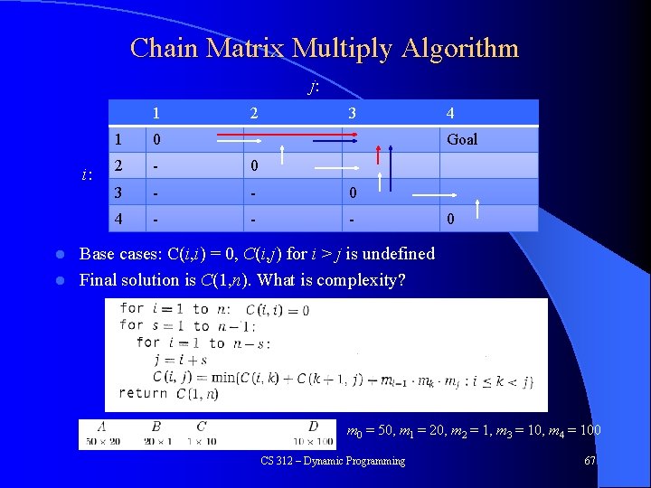
Chain Matrix Multiply Algorithm j: 1 i: 2 3 1 0 2 - 0 3 - - 0 4 - - - 4 Goal 0 Base cases: C(i, i) = 0, C(i, j) for i > j is undefined l Final solution is C(1, n). What is complexity? l m 0 = 50, m 1 = 20, m 2 = 1, m 3 = 10, m 4 = 100 CS 312 – Dynamic Programming 67

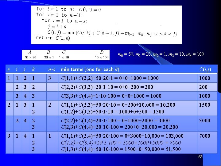
m 0 = 50, m 1 = 20, m 2 = 1, m 3 = 10, m 4 = 100 s i j k n-s min terms (one for each k) C(i, j) 3 C(1, 1)+C(2, 2)+50· 20· 1 = 0+0+1000 = 1000 2 3 2 C(2, 2)+C(3, 3)+20· 1· 10 = 0+0+200 = 200 3 4 3 C(3, 3)+C(4, 4)+1· 100 = 0+0+1000 = 1000 C(1, 1)+C(2, 3)+50· 20· 10 = 0+200+10, 000 = 10, 200 C(1, 2)+C(3, 3)+50· 1· 10 = 1000+0+500 = 1500 C(2, 2)+C(3, 4)+20· 1· 100 = 0+1000+2000 = 3000 C(2, 3)+C(4, 4)+20· 100 = 200+0+20, 000 = 20, 200 3000 C(1, 1)+C(2, 4)+50· 20· 100 = 0+3000+10, 000 = 103, 000 C(1, 2)+C(3, 4)+50· 1· 100 = 1000+5000 = 7000 C(1, 3)+C(4, 4)+50· 100 = 1500+0+50, 000 = 51, 500 7000 1 1 2 1 3 1 2 2 2 4 2 3 3 1 4 1 2 3 1 68

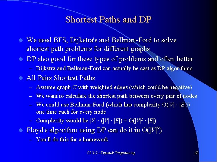
Shortest Paths and DP We used BFS, Dijkstra's and Bellman-Ford to solve shortest path problems for different graphs l DP also good for these types of problems and often better l – Dijkstra and Bellman-Ford can actually be cast as DP algorithms l All Pairs Shortest Paths – Assume graph G with weighted edges (which could be negative) – We want to calculate the shortest path between every pair of nodes – We could use Bellman-Ford (which has complexity O(|V| · |E|)) one time each for every node – Complexity would be |V| · (|V| · |E|) = O(|V|2 · |E|) l Floyd's algorithm using DP can do it in O(|V|3) – You'll do this for a homework CS 312 – Dynamic Programming 69

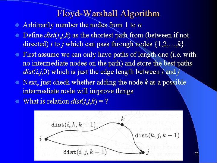
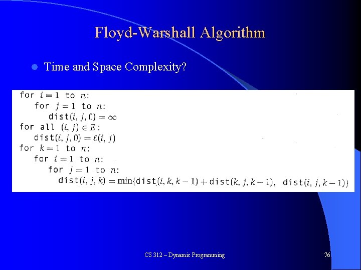
Floyd-Warshall Algorithm l l l Arbitrarily number the nodes from 1 to n Define dist(i, j, k) as the shortest path from (between if not directed) i to j which can pass through nodes {1, 2, …, k} First assume we can only have paths of length one (i. e. with no intermediate nodes on the path) and store the best paths dist(i, j, 0) which is just the edge length between i and j Next, just check whether adding the node k as a possible intermediate node will improve things What is relation dist(i, j, k) = ? CS 312 – Dynamic Programming 70

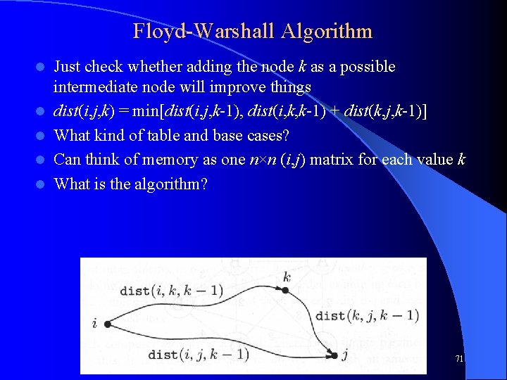
Floyd-Warshall Algorithm l l l Just check whether adding the node k as a possible intermediate node will improve things dist(i, j, k) = min[dist(i, j, k-1), dist(i, k, k-1) + dist(k, j, k-1)] What kind of table and base cases? Can think of memory as one n×n (i, j) matrix for each value k What is the algorithm? CS 312 – Dynamic Programming 71

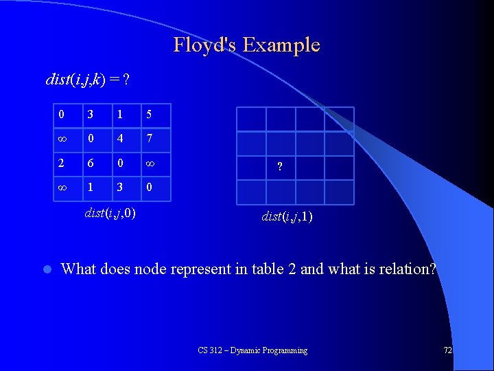
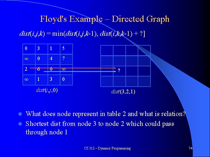
Floyd's Example dist(i, j, k) = ? 0 3 1 5 ∞ 0 4 7 2 6 0 ∞ ∞ 1 3 0 dist(i, j, 0) l ? dist(i, j, 1) What does node represent in table 2 and what is relation? CS 312 – Dynamic Programming 72

Floyd's Example – Directed Graph dist(i, j, k) = min[dist(i, j, k-1), … 0 3 1 5 ∞ 0 4 7 2 6 0 ∞ ∞ 1 3 0 dist(i, j, 0) ? dist(3, 2, 1) What does node represent in table 2 and what is relation? l Shortest dist from node 3 to node 2 which could pass through node 1 l CS 312 – Dynamic Programming 73

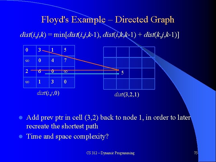
Floyd's Example – Directed Graph dist(i, j, k) = min(dist(i, j, k-1), dist(i, k, k-1) + ? ] 0 3 1 5 ∞ 0 4 7 2 6 0 ∞ ∞ 1 3 0 dist(i, j, 0) ? dist(3, 2, 1) What does node represent in table 2 and what is relation? l Shortest dist from node 3 to node 2 which could pass through node 1 l CS 312 – Dynamic Programming 74

Floyd's Example – Directed Graph dist(i, j, k) = min[dist(i, j, k-1), dist(i, k, k-1) + dist(k, j, k-1)] 0 3 1 5 ∞ 0 4 7 2 6 0 ∞ ∞ 1 3 0 dist(i, j, 0) 5 dist(3, 2, 1) Add prev ptr in cell (3, 2) back to node 1, in order to later recreate the shortest path l Time and space complexity? l CS 312 – Dynamic Programming 75

Floyd-Warshall Algorithm l Time and Space Complexity? CS 312 – Dynamic Programming 76

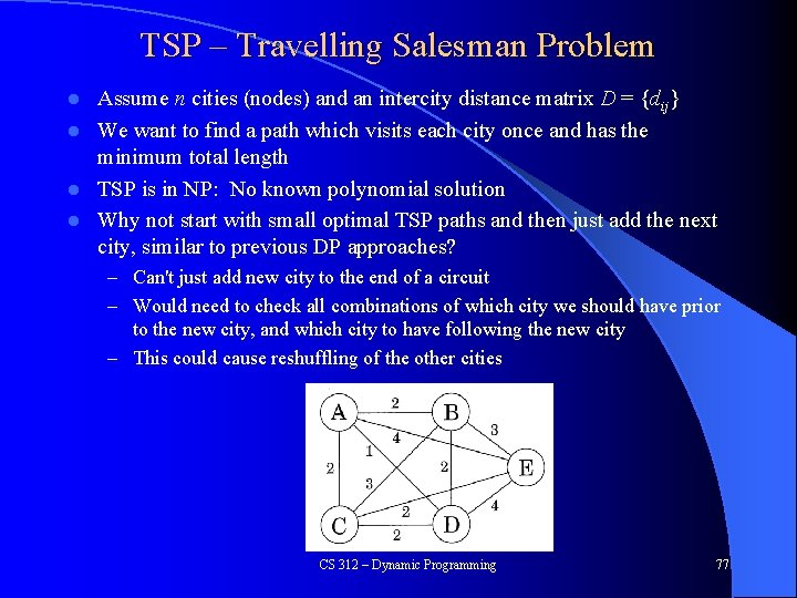
TSP – Travelling Salesman Problem Assume n cities (nodes) and an intercity distance matrix D = {dij} l We want to find a path which visits each city once and has the minimum total length l TSP is in NP: No known polynomial solution l Why not start with small optimal TSP paths and then just add the next city, similar to previous DP approaches? l – Can't just add new city to the end of a circuit – Would need to check all combinations of which city we should have prior to the new city, and which city to have following the new city – This could cause reshuffling of the other cities CS 312 – Dynamic Programming 77

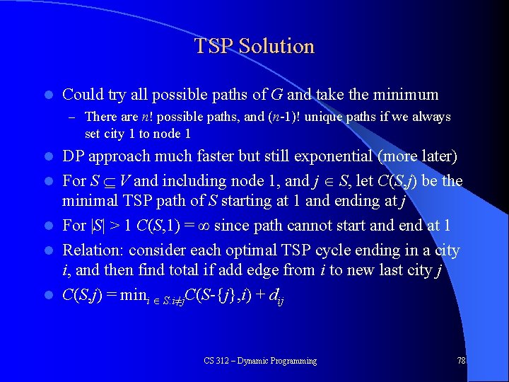
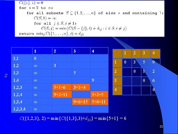
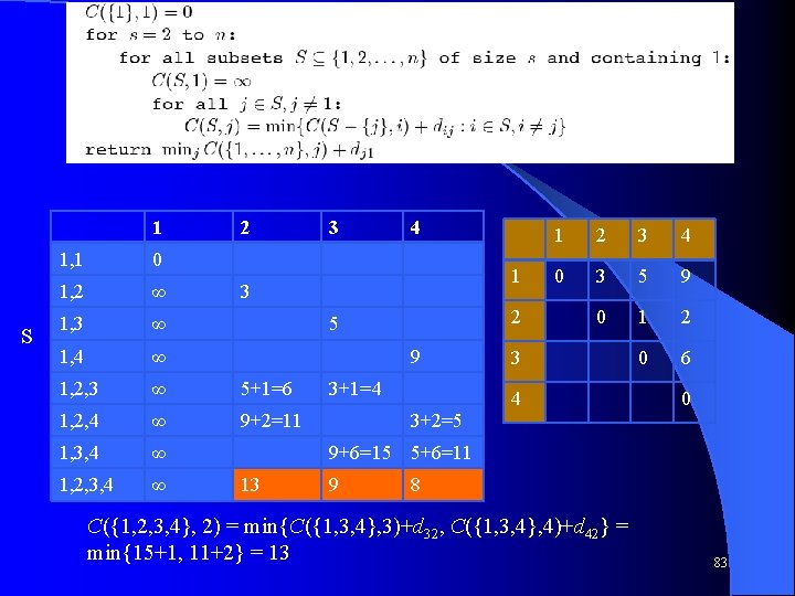
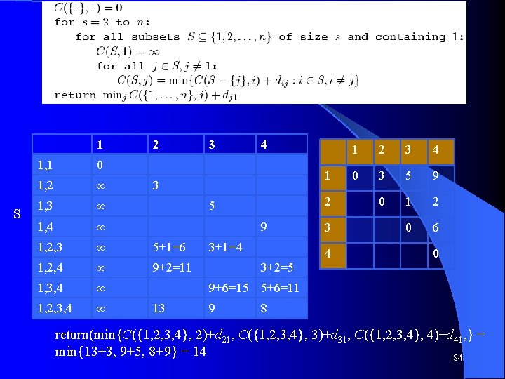
TSP Solution l Could try all possible paths of G and take the minimum – There are n! possible paths, and (n-1)! unique paths if we always set city 1 to node 1 l l l DP approach much faster but still exponential (more later) For S V and including node 1, and j S, let C(S, j) be the minimal TSP path of S starting at 1 and ending at j For |S| > 1 C(S, 1) = ∞ since path cannot start and end at 1 Relation: consider each optimal TSP cycle ending in a city i, and then find total if add edge from i to new last city j C(S, j) = mini S: i≠j. C(S-{j}, i) + dij CS 312 – Dynamic Programming 78

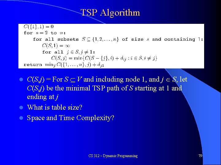
TSP Algorithm C(S, j) = For S V and including node 1, and j S, let C(S, j) be the minimal TSP path of S starting at 1 and ending at j l What is table size? l Space and Time Complexity? l CS 312 – Dynamic Programming 79

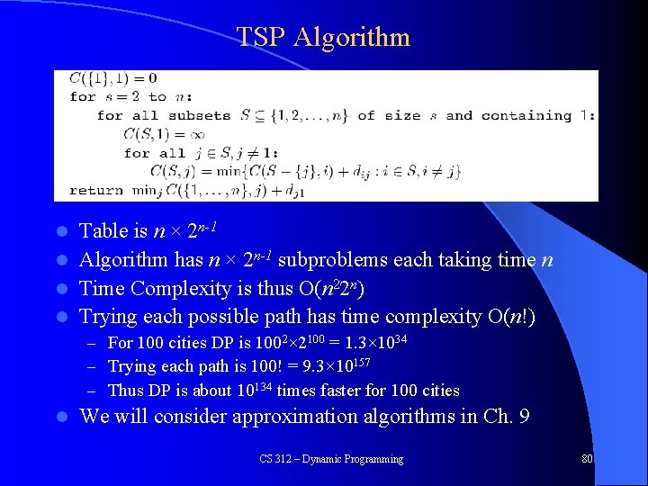
TSP Algorithm Table is n × 2 n-1 l Algorithm has n × 2 n-1 subproblems each taking time n l Time Complexity is thus O(n 22 n) l Trying each possible path has time complexity O(n!) l – For 100 cities DP is 1002× 2100 = 1. 3× 1034 – Trying each path is 100! = 9. 3× 10157 – Thus DP is about 10134 times faster for 100 cities l We will consider approximation algorithms in Ch. 9 CS 312 – Dynamic Programming 80

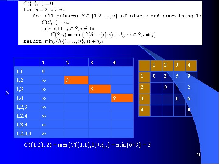
l sdfsdf 1 S 1, 1 0 1, 2 ∞ 1, 3 ∞ 1, 4 ∞ 1, 2, 3 ∞ 1, 2, 4 ∞ 1, 3, 4 ∞ 1, 2, 3, 4 ∞ 2 3 4 1 3 2 5 9 3 4 1 2 3 4 0 3 5 9 0 1 2 0 6 0 C({1, 2}, 2) = min{C({1, 1}, 1)+d 12} = min{0+3} = 3 81

l sdfsdf 1 S 2 1, 1 0 1, 2 ∞ 1, 3 ∞ 1, 4 ∞ 1, 2, 3 ∞ 5+1=6 1, 2, 4 ∞ 9+2=11 1, 3, 4 ∞ 1, 2, 3, 4 ∞ 3 4 1 3 1 2 3 4 0 3 5 9 0 1 2 0 6 2 5 9 3+1=4 3 4 0 3+2=5 9+6=15 5+6=11 C({1, 2, 3}, 2) = min{C({1, 3}, 3)+d 32} = min{5+1} = 6 82

l sdfsdf 1 S 2 1, 1 0 1, 2 ∞ 1, 3 ∞ 1, 4 ∞ 1, 2, 3 ∞ 5+1=6 1, 2, 4 ∞ 9+2=11 1, 3, 4 ∞ 1, 2, 3, 4 ∞ 3 4 1 3 2 5 9 3+1=4 1 2 3 4 0 3 5 9 0 1 2 0 6 3 4 0 3+2=5 9+6=15 5+6=11 13 9 8 C({1, 2, 3, 4}, 2) = min{C({1, 3, 4}, 3)+d 32, C({1, 3, 4}, 4)+d 42} = min{15+1, 11+2} = 13 83

l sdfsdf 1 S 2 1, 1 0 1, 2 ∞ 1, 3 ∞ 1, 4 ∞ 1, 2, 3 ∞ 5+1=6 1, 2, 4 ∞ 9+2=11 1, 3, 4 ∞ 1, 2, 3, 4 ∞ 3 4 1 3 2 5 9 3+1=4 3 4 1 2 3 4 0 3 5 9 0 1 2 0 6 0 3+2=5 9+6=15 5+6=11 13 9 8 return(min{C({1, 2, 3, 4}, 2)+d 21, C({1, 2, 3, 4}, 3)+d 31, C({1, 2, 3, 4}, 4)+d 41, } = min{13+3, 9+5, 8+9} = 14 84

Using Dynamic Programming Many applications can gain efficiency by using Dynamic Programming l Works when there are overlapping subproblems l – The recursive approach would lead to much duplicate work l And when subproblems (given by a recursive definition and DAG dependencies) are only slightly (constant factor) smaller than the original problem – If smaller by a multiplicative factor, consider divide and conquer CS 312 – Dynamic Programming 85

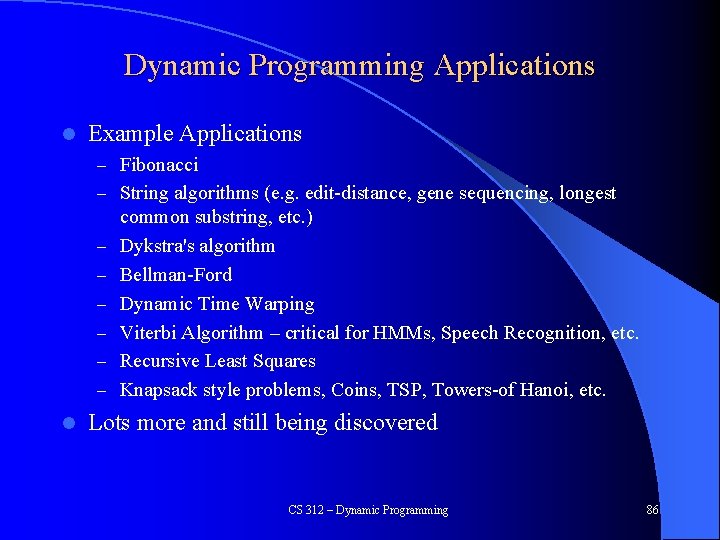
Dynamic Programming Applications l Example Applications – Fibonacci – String algorithms (e. g. edit-distance, gene sequencing, longest – – – l common substring, etc. ) Dykstra's algorithm Bellman-Ford Dynamic Time Warping Viterbi Algorithm – critical for HMMs, Speech Recognition, etc. Recursive Least Squares Knapsack style problems, Coins, TSP, Towers-of Hanoi, etc. Lots more and still being discovered CS 312 – Dynamic Programming 86