Divideandconquer United we shall prevail Divide we shall

![Tiling a defective chessboard n Let array Board denotes chessboard, Board[0][0] denotes the position Tiling a defective chessboard n Let array Board denotes chessboard, Board[0][0] denotes the position](https://slidetodoc.com/presentation_image_h/ad88a6b3dc70119bd84d89909a175dc1/image-53.jpg)
- Slides: 57

Divide-and-conquer “United, we shall prevail; Divide, we shall perish”

5. 1 Divide-and-conquer n n Many useful algorithms are recursive in structure: to solve a given problem, they call themselves recursively one or more times to deal with closely related subproblems. Divide-and-conquer approach: they break the problem into several subproblems that are similar to the original problem but smaller in size, solve the subproblems recursively, and then combine these solutions to create a solution to the original problem. 2

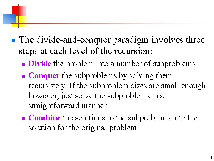
n The divide-and-conquer paradigm involves three steps at each level of the recursion: n n n Divide the problem into a number of subproblems. Conquer the subproblems by solving them recursively. If the subproblem sizes are small enough, however, just solve the subproblems in a straightforward manner. Combine the solutions to the subproblems into the solution for the original problem. 3

Analyzing divide-and-conquer algorithms n n When an algorithm contains a recursive call to itself, its running time can often be described by a recurrence equation or recurrence, which describes the overall running time on a problem of size n in terms of the running time on smaller inputs. We can then use mathematical tools to solve the recurrence and provide bounds on the performance of the algorithm. One advantage of divide-and-conquer algorithms is that their running times are often easily determined using techniques that will be introduced in section 6. 4

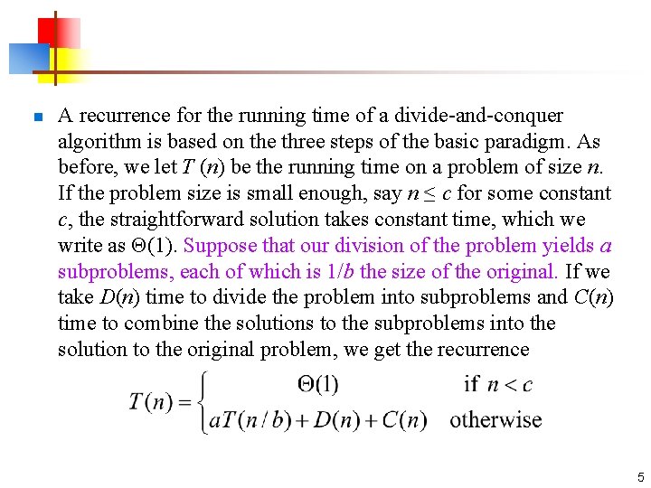
n A recurrence for the running time of a divide-and-conquer algorithm is based on the three steps of the basic paradigm. As before, we let T (n) be the running time on a problem of size n. If the problem size is small enough, say n ≤ c for some constant c, the straightforward solution takes constant time, which we write as Θ(1). Suppose that our division of the problem yields a subproblems, each of which is 1/b the size of the original. If we take D(n) time to divide the problem into subproblems and C(n) time to combine the solutions to the subproblems into the solution to the original problem, we get the recurrence 5

5. 2 Merge sort for the sorting problem n The basic steps of the merge sort algorithm: n Divide the n-element sequence to be sorted into two subsequences of n/2 elements each. n Sort the two subsequences recursively using merge sort. n Merge the two sorted subsequences to produce the sorted answer. 6

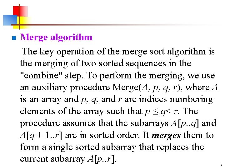
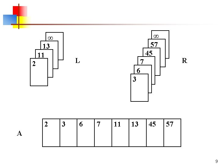
n Merge algorithm The key operation of the merge sort algorithm is the merging of two sorted sequences in the "combine" step. To perform the merging, we use an auxiliary procedure Merge(A, p, q, r), where A is an array and p, q, and r are indices numbering elements of the array such that p ≤ q< r. The procedure assumes that the subarrays A[p. . q] and A[q + 1. . r] are in sorted order. It merges them to form a single sorted subarray that replaces the current subarray A[p. . r]. 7

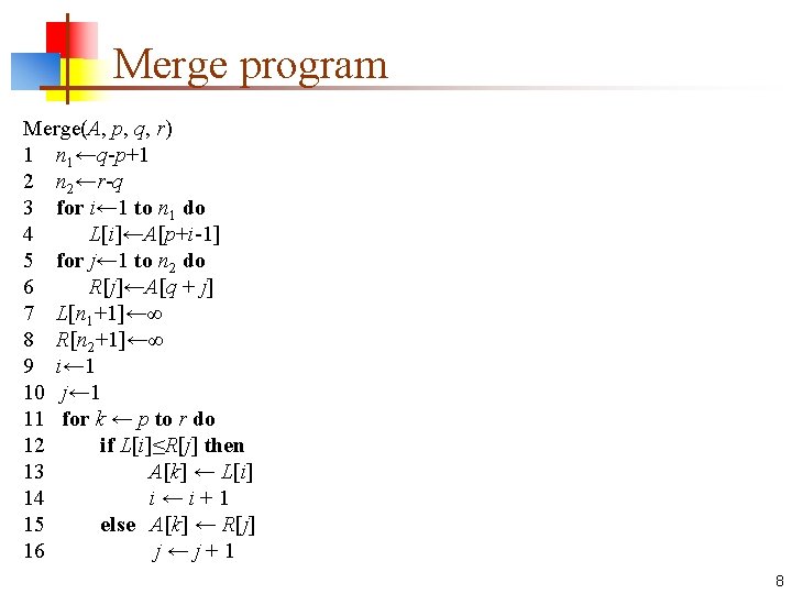
Merge program Merge(A, p, q, r) 1 n 1←q-p+1 2 n 2←r-q 3 for i← 1 to n 1 do 4 L[i]←A[p+i-1] 5 for j← 1 to n 2 do 6 R[j]←A[q + j] 7 L[n 1+1]←∞ 8 R[n 2+1]←∞ 9 i← 1 10 j← 1 11 for k ← p to r do 12 if L[i]≤R[j] then 13 A[k] ← L[i] 14 i←i+1 15 else A[k] ← R[j] 16 j←j+1 8

∞ 13 11 L 2 2 ∞ 57 45 3 6 R 7 6 3 7 11 13 45 57 A 9

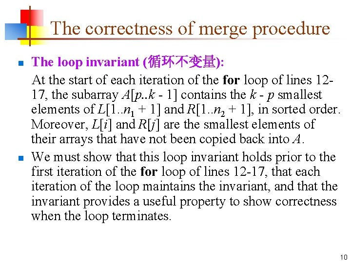
The correctness of merge procedure n n The loop invariant (循环不变量): At the start of each iteration of the for loop of lines 1217, the subarray A[p. . k - 1] contains the k - p smallest elements of L[1. . n 1 + 1] and R[1. . n 2 + 1], in sorted order. Moreover, L[i] and R[j] are the smallest elements of their arrays that have not been copied back into A. We must show that this loop invariant holds prior to the first iteration of the for loop of lines 12 -17, that each iteration of the loop maintains the invariant, and that the invariant provides a useful property to show correctness when the loop terminates. 10

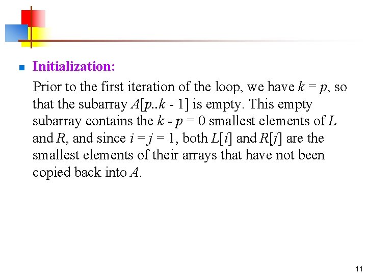
n Initialization: Prior to the first iteration of the loop, we have k = p, so that the subarray A[p. . k - 1] is empty. This empty subarray contains the k - p = 0 smallest elements of L and R, and since i = j = 1, both L[i] and R[j] are the smallest elements of their arrays that have not been copied back into A. 11

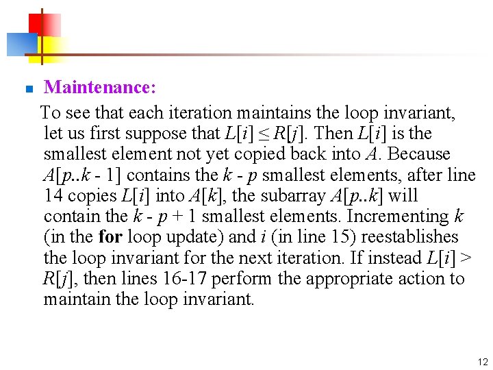
n Maintenance: To see that each iteration maintains the loop invariant, let us first suppose that L[i] ≤ R[j]. Then L[i] is the smallest element not yet copied back into A. Because A[p. . k - 1] contains the k - p smallest elements, after line 14 copies L[i] into A[k], the subarray A[p. . k] will contain the k - p + 1 smallest elements. Incrementing k (in the for loop update) and i (in line 15) reestablishes the loop invariant for the next iteration. If instead L[i] > R[j], then lines 16 -17 perform the appropriate action to maintain the loop invariant. 12

n Termination: At termination, k = r + 1. By the loop invariant, the subarray A[p. . k -1], which is A[p. . r], contains the k - p = r - p + 1 smallest elements of L[1. . n 1 + 1] and R[1. . n 2 + 1], in sorted order. The arrays L and R together contain n 1 + n 2 + 2 = r- p + 3 elements. All but the two largest have been copied back into A, and these two largest elements are the sentinels. 13

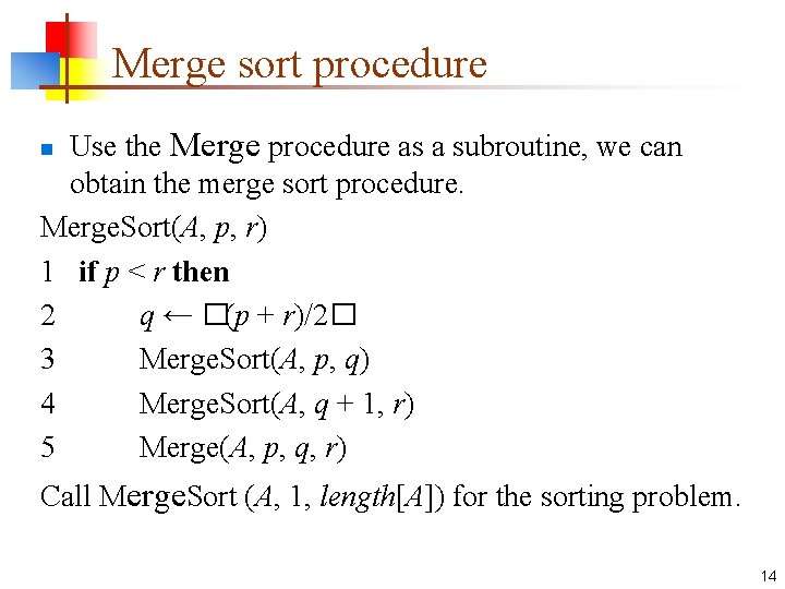
Merge sort procedure Use the Merge procedure as a subroutine, we can obtain the merge sort procedure. Merge. Sort(A, p, r) 1 if p < r then 2 q ← �(p + r)/2� 3 Merge. Sort(A, p, q) 4 Merge. Sort(A, q + 1, r) 5 Merge(A, p, q, r) n Call Merge. Sort (A, 1, length[A]) for the sorting problem. 14

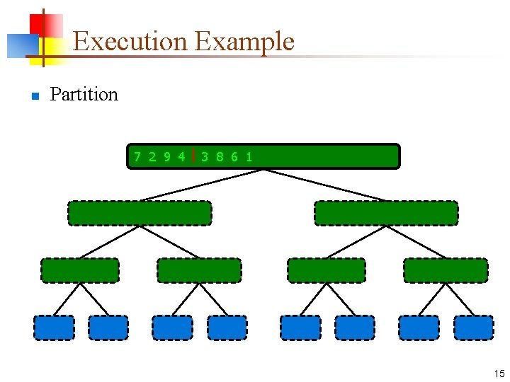
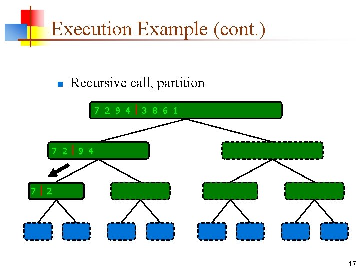
Execution Example n Partition 7 2 9 4 3 8 6 1 1 2 3 4 6 7 8 9 7 2 9 4 2 4 7 9 7 2 2 7 7 7 2 2 3 8 6 1 1 3 8 6 9 4 4 9 9 9 4 4 3 8 3 3 8 8 6 1 1 6 6 6 1 1 15

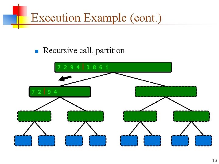
Execution Example (cont. ) n Recursive call, partition 7 2 9 4 3 8 6 1 1 2 3 4 6 7 8 9 7 2 9 4 2 4 7 9 7 2 2 7 7 7 2 2 3 8 6 1 1 3 8 6 9 4 4 9 9 9 4 4 3 8 3 3 8 8 6 1 1 6 6 6 1 1 16

Execution Example (cont. ) n Recursive call, partition 7 2 9 4 3 8 6 1 1 2 3 4 6 7 8 9 7 2 9 4 2 4 7 9 7 2 2 7 7 7 2 2 3 8 6 1 1 3 8 6 9 4 4 9 9 9 4 4 3 8 3 3 8 8 6 1 1 6 6 6 1 1 17

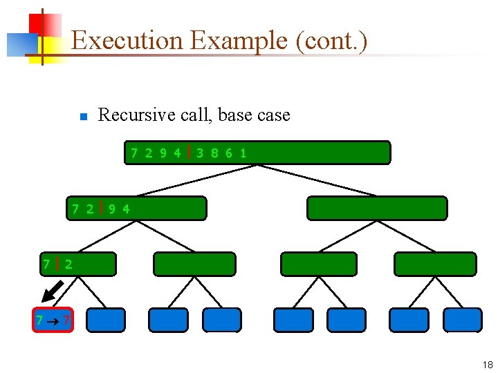
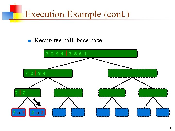
Execution Example (cont. ) n Recursive call, base case 7 2 9 4 3 8 6 1 1 2 3 4 6 7 8 9 7 2 9 4 2 4 7 9 7 2 2 7 7 7 2 2 3 8 6 1 1 3 8 6 9 4 4 9 9 9 4 4 3 8 3 3 8 8 6 1 1 6 6 6 1 1 18

Execution Example (cont. ) n Recursive call, base case 7 2 9 4 3 8 6 1 1 2 3 4 6 7 8 9 7 2 9 4 2 4 7 9 7 2 2 7 7 7 2 2 3 8 6 1 1 3 8 6 9 4 4 9 9 9 4 4 3 8 3 3 8 8 6 1 1 6 6 6 1 1 19

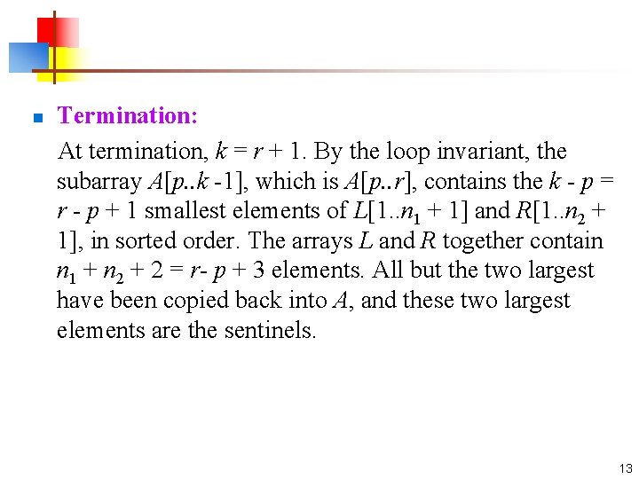
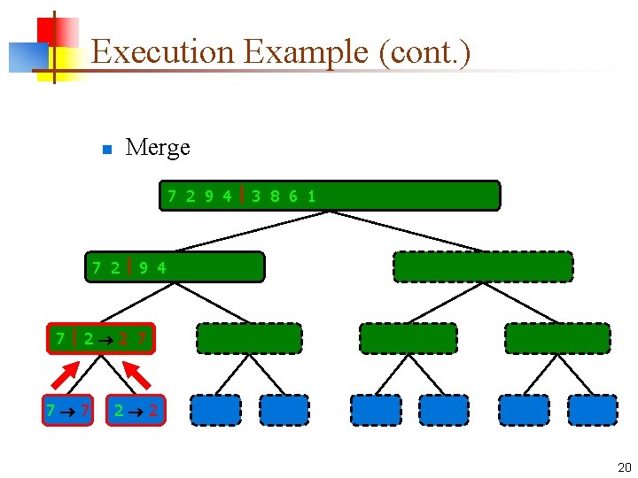
Execution Example (cont. ) n Merge 7 2 9 4 3 8 6 1 1 2 3 4 6 7 8 9 7 2 9 4 2 4 7 9 7 2 2 7 7 7 2 2 3 8 6 1 1 3 8 6 9 4 4 9 9 9 4 4 3 8 3 3 8 8 6 1 1 6 6 6 1 1 20

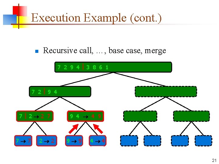
Execution Example (cont. ) n Recursive call, …, base case, merge 7 2 9 4 3 8 6 1 1 2 3 4 6 7 8 9 7 2 9 4 2 4 7 9 7 2 2 7 7 7 2 2 3 8 6 1 1 3 8 6 9 4 4 9 9 9 4 4 3 8 3 3 8 8 6 1 1 6 6 6 1 1 21

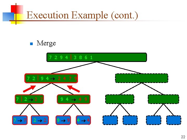
Execution Example (cont. ) n Merge 7 2 9 4 3 8 6 1 1 2 3 4 6 7 8 9 7 2 9 4 2 4 7 9 7 2 2 7 7 7 2 2 3 8 6 1 1 3 8 6 9 4 4 9 9 9 4 4 3 8 3 3 8 8 6 1 1 6 6 6 1 1 22

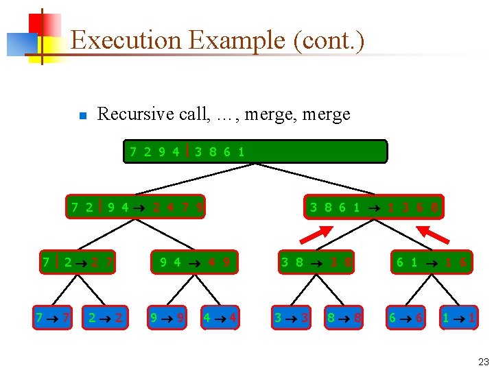
Execution Example (cont. ) n Recursive call, …, merge 7 2 9 4 3 8 6 1 1 2 3 4 6 7 8 9 7 2 9 4 2 4 7 9 7 2 2 7 7 7 2 2 3 8 6 1 1 3 6 8 9 4 4 9 9 9 4 4 3 8 3 3 8 8 6 1 1 6 6 6 1 1 23

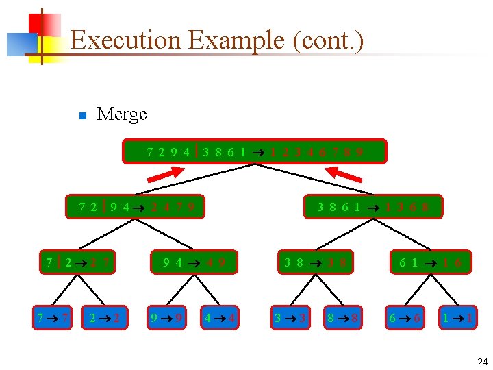
Execution Example (cont. ) n Merge 7 2 9 4 3 8 6 1 1 2 3 4 6 7 8 9 7 2 9 4 2 4 7 9 7 2 2 7 7 7 2 2 3 8 6 1 1 3 6 8 9 4 4 9 9 9 4 4 3 8 3 3 8 8 6 1 1 6 6 6 1 1 24

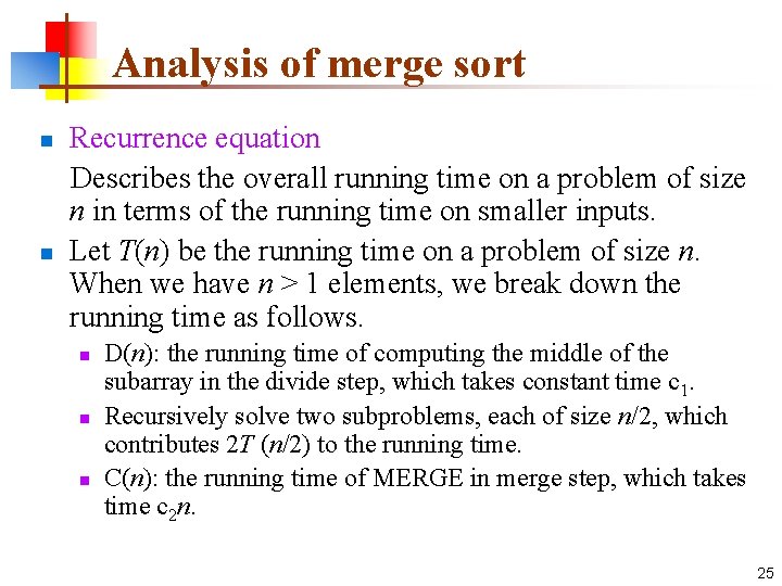
Analysis of merge sort n n Recurrence equation Describes the overall running time on a problem of size n in terms of the running time on smaller inputs. Let T(n) be the running time on a problem of size n. When we have n > 1 elements, we break down the running time as follows. n n n D(n): the running time of computing the middle of the subarray in the divide step, which takes constant time c 1. Recursively solve two subproblems, each of size n/2, which contributes 2 T (n/2) to the running time. C(n): the running time of MERGE in merge step, which takes time c 2 n. 25

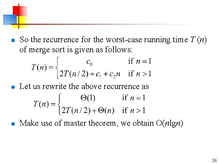
n So the recurrence for the worst-case running time T (n) of merge sort is given as follows: n Let us rewrite the above recurrence as n Make use of master theorem, we obtain O(nlgn) 26

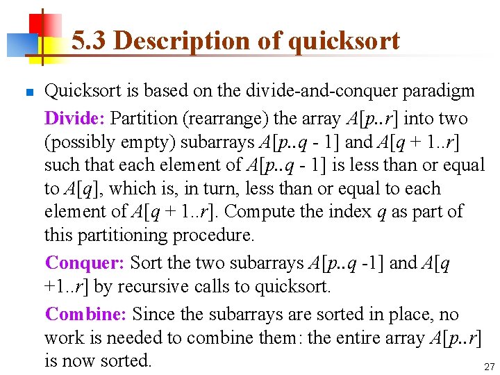
5. 3 Description of quicksort n Quicksort is based on the divide-and-conquer paradigm Divide: Partition (rearrange) the array A[p. . r] into two (possibly empty) subarrays A[p. . q - 1] and A[q + 1. . r] such that each element of A[p. . q - 1] is less than or equal to A[q], which is, in turn, less than or equal to each element of A[q + 1. . r]. Compute the index q as part of this partitioning procedure. Conquer: Sort the two subarrays A[p. . q -1] and A[q +1. . r] by recursive calls to quicksort. Combine: Since the subarrays are sorted in place, no work is needed to combine them: the entire array A[p. . r] is now sorted. 27

C. Antony R. Hoare United Kingdom – 1980 http: //amturing. acm. org/award_ winners/hoare_4622167. cfm 28

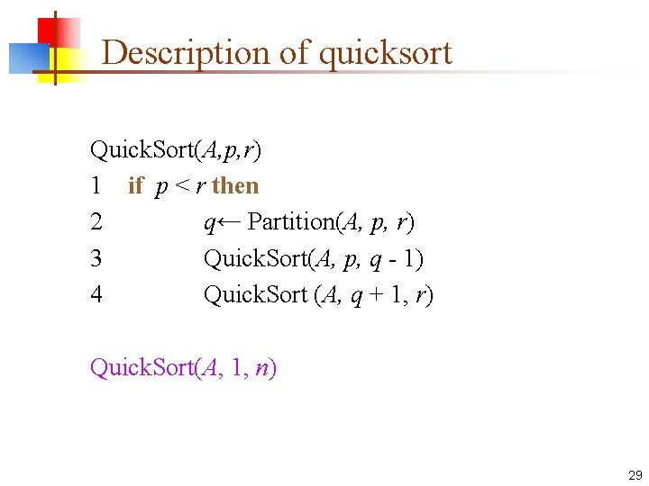
Description of quicksort Quick. Sort(A, p, r) 1 if p < r then 2 q← Partition(A, p, r) 3 Quick. Sort(A, p, q - 1) 4 Quick. Sort (A, q + 1, r) Quick. Sort(A, 1, n) 29

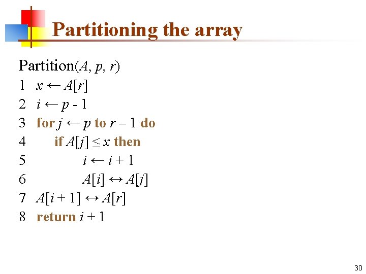
Partitioning the array Partition(A, p, r) 1 2 3 4 5 6 7 8 x ← A[r] i←p-1 for j ← p to r – 1 do if A[j] ≤ x then i←i+1 A[i] ↔ A[j] A[i + 1] ↔ A[r] return i + 1 30

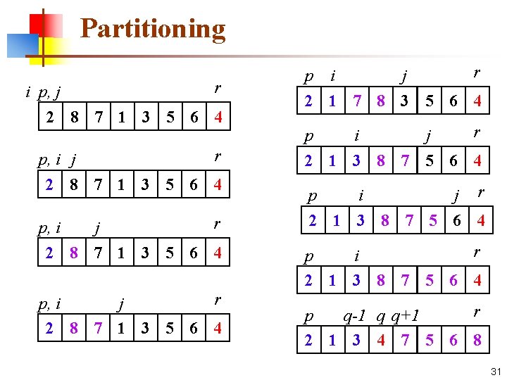
Partitioning r i p, j 2 8 7 1 3 5 6 4 r p, i j 2 8 7 1 3 5 6 4 r p i j 2 1 7 8 3 5 6 4 r p i j 2 1 3 8 7 5 6 4 p i j r 2 1 3 8 7 5 6 4 r p i 2 1 3 8 7 5 6 4 r p q-1 q q+1 2 1 3 4 7 5 6 8 31

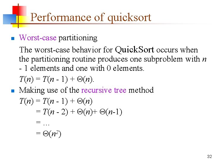
Performance of quicksort n n Worst-case partitioning The worst-case behavior for Quick. Sort occurs when the partitioning routine produces one subproblem with n - 1 elements and one with 0 elements. T(n) = T(n - 1) + Θ(n). Making use of the recursive tree method T(n) = T(n - 1) + Θ(n) = T(n - 2) + Θ(n)+ Θ(n-1) =… = Θ(n 2) 32

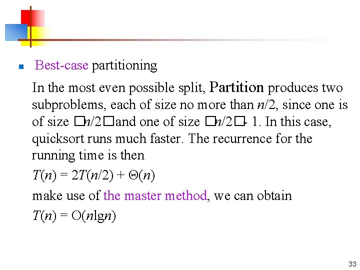
n Best-case partitioning In the most even possible split, Partition produces two subproblems, each of size no more than n/2, since one is of size �n/2�and one of size �n/2�- 1. In this case, quicksort runs much faster. The recurrence for the running time is then T(n) = 2 T(n/2) + Θ(n) make use of the master method, we can obtain T(n) = O(nlgn) 33

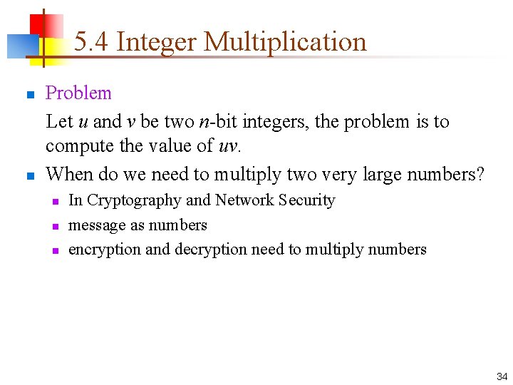
5. 4 Integer Multiplication n n Problem Let u and v be two n-bit integers, the problem is to compute the value of uv. When do we need to multiply two very large numbers? n n n In Cryptography and Network Security message as numbers encryption and decryption need to multiply numbers 34

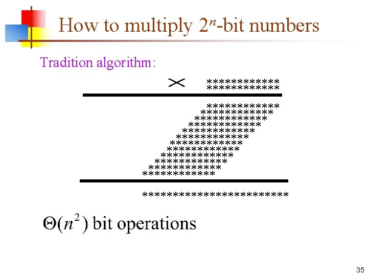
How to multiply 2 n-bit numbers Tradition algorithm: ************ ************ ************ ************ 35

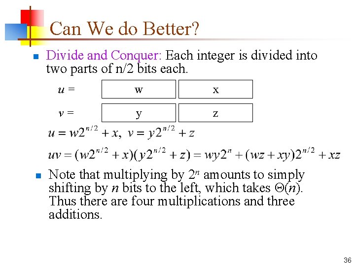
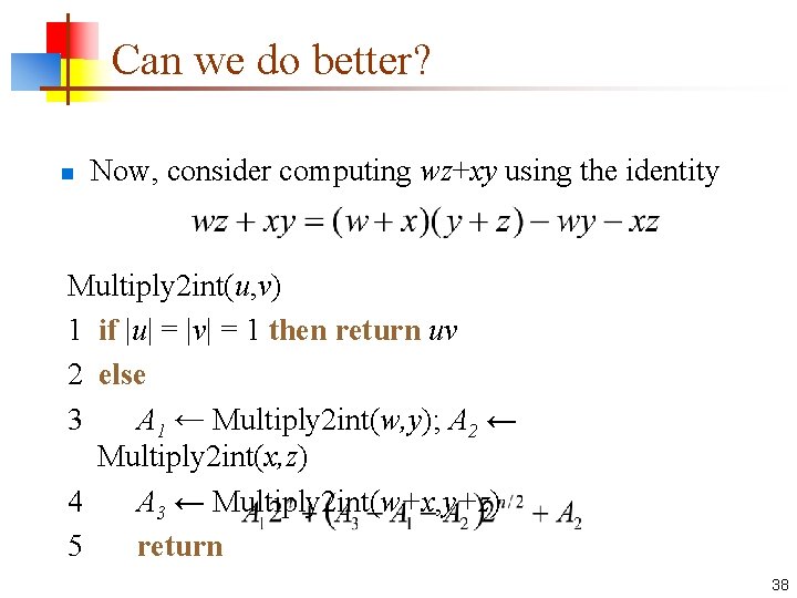
Can We do Better? n n Divide and Conquer: Each integer is divided into two parts of n/2 bits each. u= w x v= y z Note that multiplying by 2 n amounts to simply shifting by n bits to the left, which takes Θ(n). Thus there are four multiplications and three additions. 36

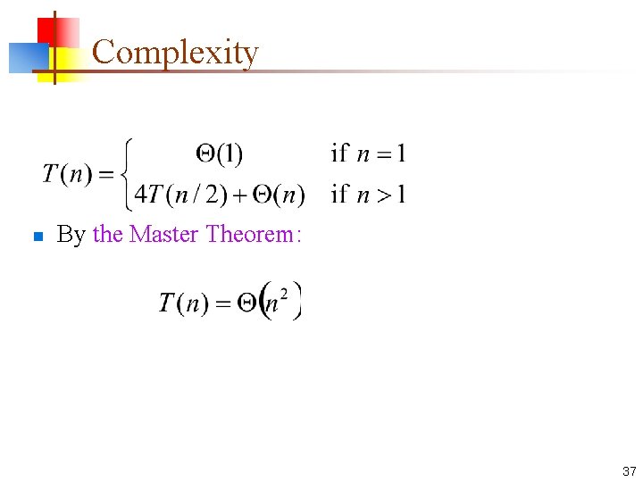
Complexity n By the Master Theorem: 37

Can we do better? n Now, consider computing wz+xy using the identity Multiply 2 int(u, v) 1 if |u| = |v| = 1 then return uv 2 else 3 A 1 ← Multiply 2 int(w, y); A 2 ← Multiply 2 int(x, z) 4 A 3 ← Multiply 2 int(w+x, y+z) 5 return 38

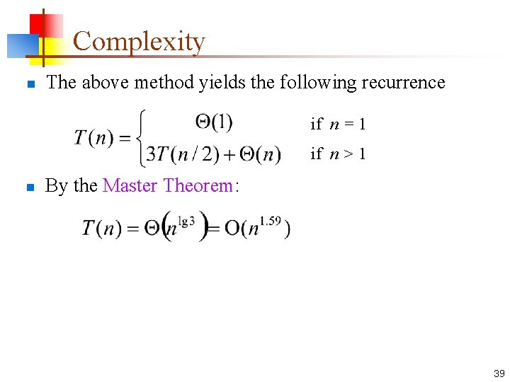
Complexity n The above method yields the following recurrence if n = 1 if n > 1 n By the Master Theorem: 39

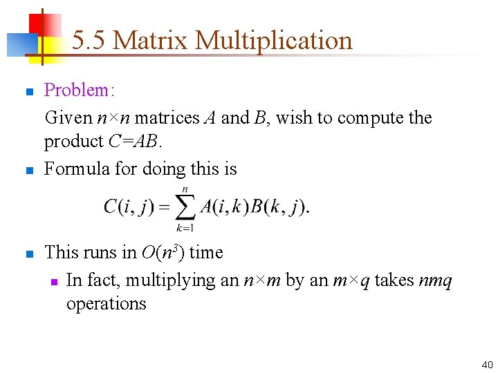
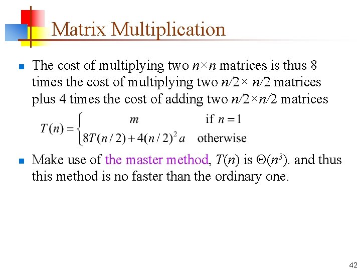
5. 5 Matrix Multiplication n Problem: Given n×n matrices A and B, wish to compute the product C=AB. Formula for doing this is This runs in O(n 3) time n In fact, multiplying an n×m by an m×q takes nmq operations 40

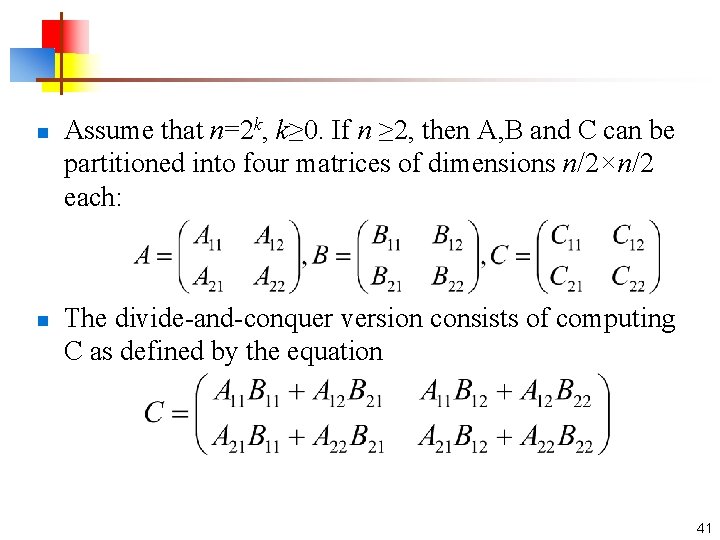
n n Assume that n=2 k, k≥ 0. If n ≥ 2, then A, B and C can be partitioned into four matrices of dimensions n/2×n/2 each: The divide-and-conquer version consists of computing C as defined by the equation 41

Matrix Multiplication n n The cost of multiplying two n×n matrices is thus 8 times the cost of multiplying two n/2× n/2 matrices plus 4 times the cost of adding two n/2×n/2 matrices Make use of the master method, T(n) is Θ(n 3). and thus this method is no faster than the ordinary one. 42

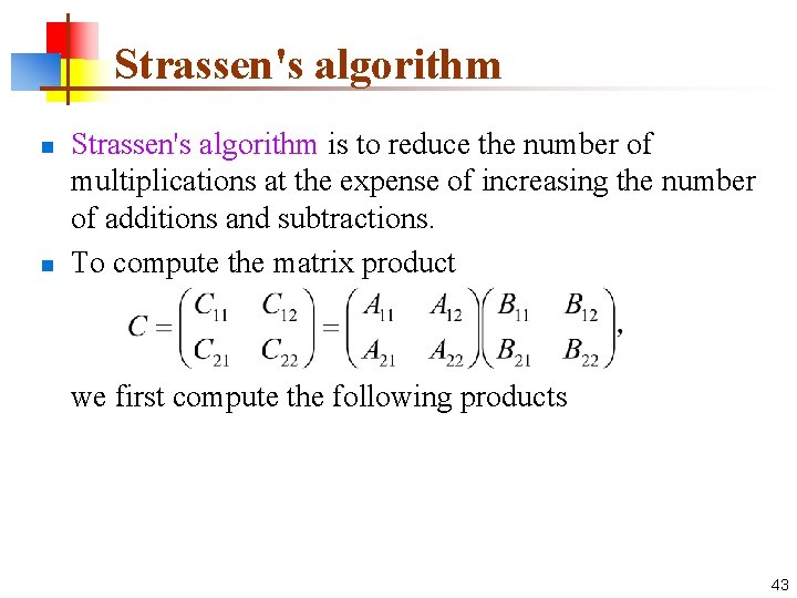
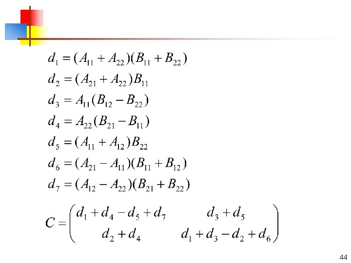
Strassen's algorithm n n Strassen's algorithm is to reduce the number of multiplications at the expense of increasing the number of additions and subtractions. To compute the matrix product we first compute the following products 43

44

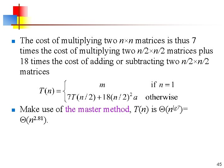
n n The cost of multiplying two n×n matrices is thus 7 times the cost of multiplying two n/2×n/2 matrices plus 18 times the cost of adding or subtracting two n/2×n/2 matrices Make use of the master method, T(n) is Θ(nlg 7)= Θ(n 2. 81). 45

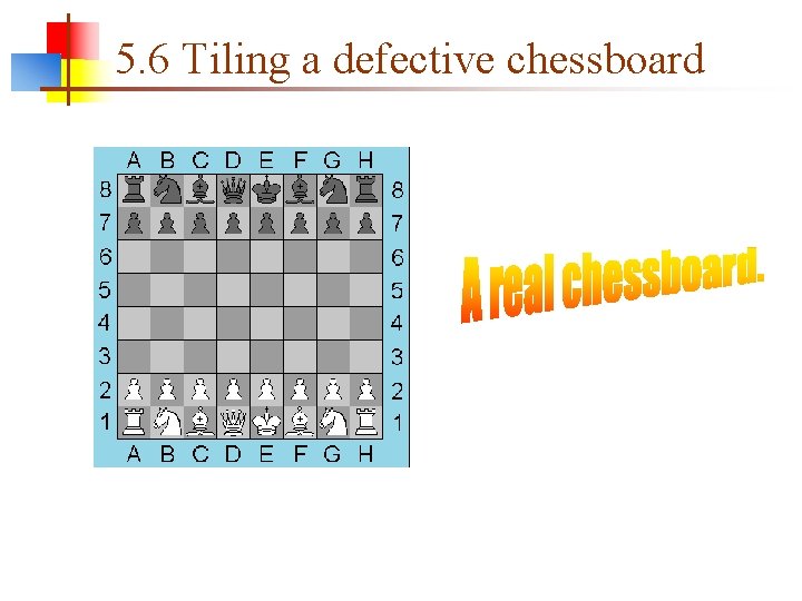
5. 6 Tiling a defective chessboard

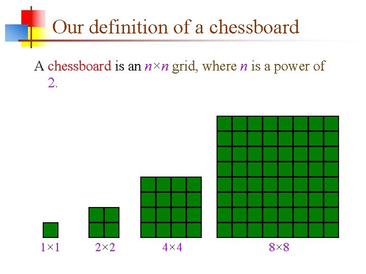
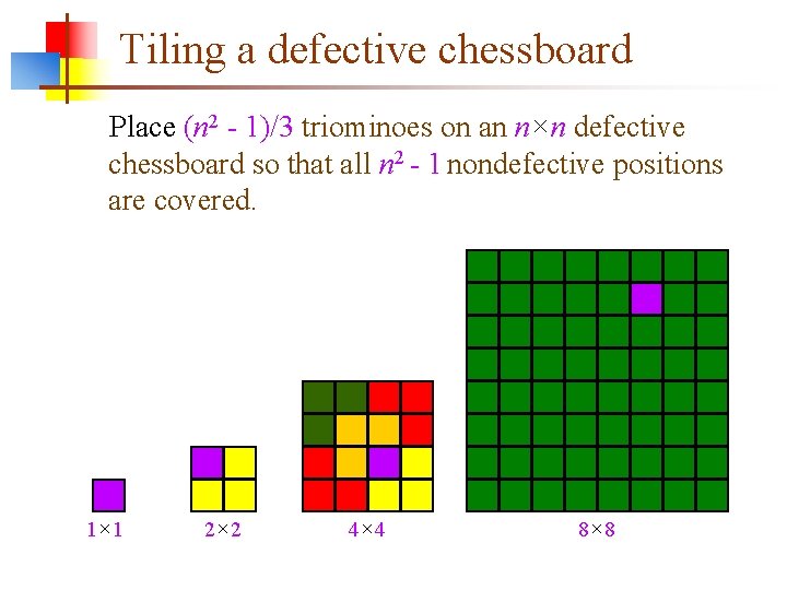
Our definition of a chessboard A chessboard is an n×n grid, where n is a power of 2. 1× 1 2× 2 4× 4 8× 8

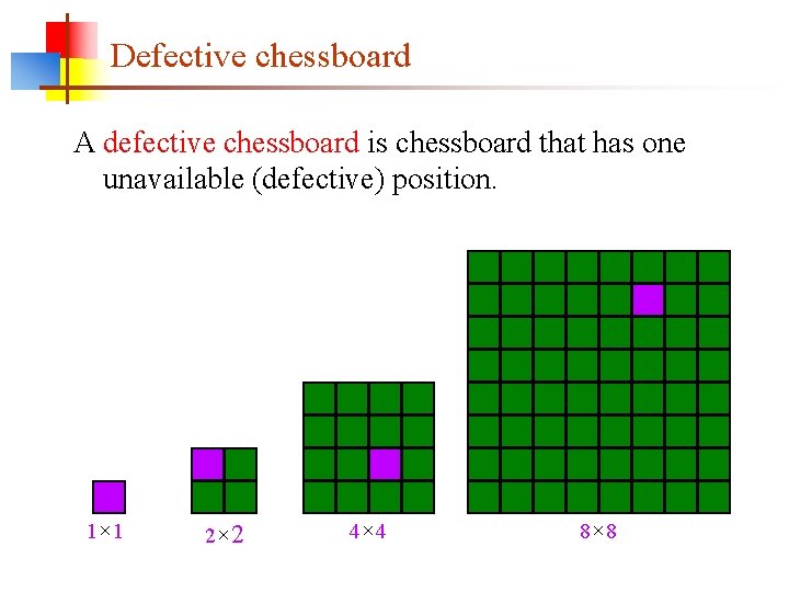
Defective chessboard A defective chessboard is chessboard that has one unavailable (defective) position. 1× 1 2× 2 4× 4 8× 8

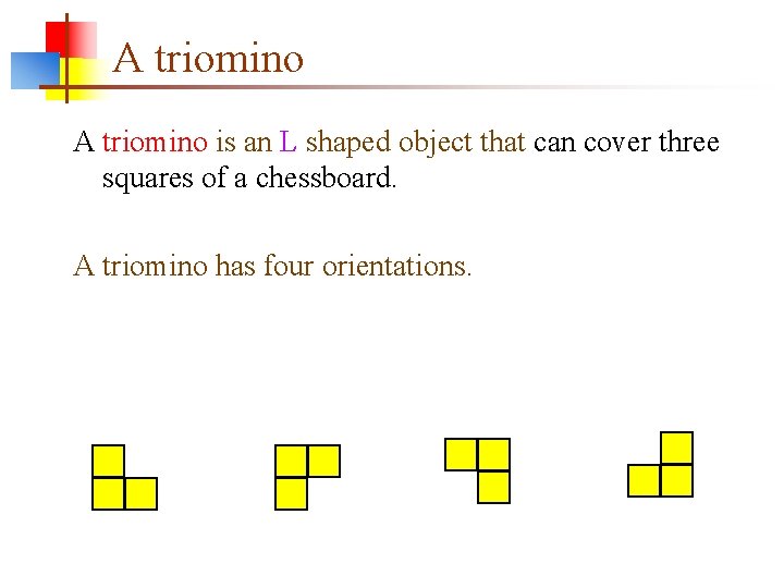
A triomino is an L shaped object that can cover three squares of a chessboard. A triomino has four orientations.

Tiling a defective chessboard Place (n 2 - 1)/3 triominoes on an n×n defective chessboard so that all n 2 - 1 nondefective positions are covered. 1× 1 2× 2 4× 4 8× 8

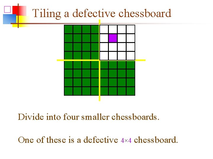
Tiling a defective chessboard Divide into four smaller chessboards. One of these is a defective 4× 4 chessboard.

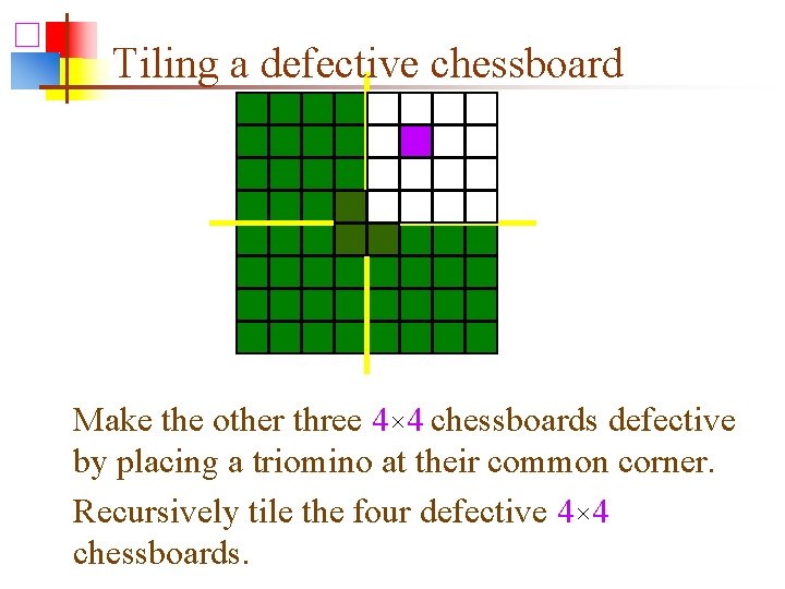
Tiling a defective chessboard Make the other three 4× 4 chessboards defective by placing a triomino at their common corner. Recursively tile the four defective 4× 4 chessboards.
![Tiling a defective chessboard n Let array Board denotes chessboard Board00 denotes the position Tiling a defective chessboard n Let array Board denotes chessboard, Board[0][0] denotes the position](https://slidetodoc.com/presentation_image_h/ad88a6b3dc70119bd84d89909a175dc1/image-53.jpg)
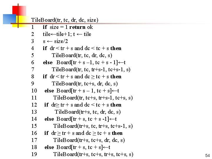
Tiling a defective chessboard n Let array Board denotes chessboard, Board[0][0] denotes the position of left-upper corner, tile denotes the number of triomino,tr denotes the row position of left-upper square in chessboard, tc denotes the column position of left-upper square in chessboard,(dr, dl) denotes the position (row, column) of defective square, size denotes the row or column number of chessboard.

Tile. Board(tr, tc, dr, dc, size) 1 if size = 1 return ok 2 tile←tile+1; t ← tile 3 s ← size/2 4 if dr < tr + s and dc < tc + s then 5 Tile. Board(tr, tc, dr, dc, s) 6 else Board[tr + s – 1, tc + s - 1]←t 7 Tile. Board(tr, tc, tr+s-1, tc+s-1, s) 8 if dr < tr + s and dc ≥ tc + s then 9 Tile. Board(tr, tc+s, dr, dc, s) 10 else Board[tr + s – 1, tc + s]←t 11 Tile. Board(tr, tc+s, tr+s-1, tc+s, s) 12 if dr≥ tr + s and dc < tc + s then 13 Tile. Board(tr+s, tc, dr, dc, s) 14 else Board[tr + s, tc + s -1]←t 15 Tile. Board(tr+s, tc, tr+s, tc+s-1, s) 16 if dr ≥ tr + s and dc ≥ tc + s then 17 Tile. Board(tr+s, tc+s, dr, dc, s) 18 else Board[tr + s, tc + s]←t 19 Tile. Board(tr+s, tc+s, s) 54

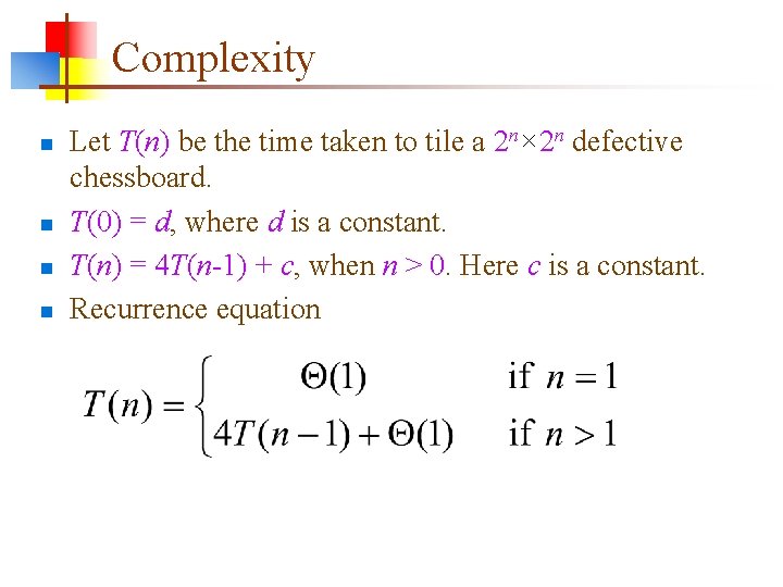
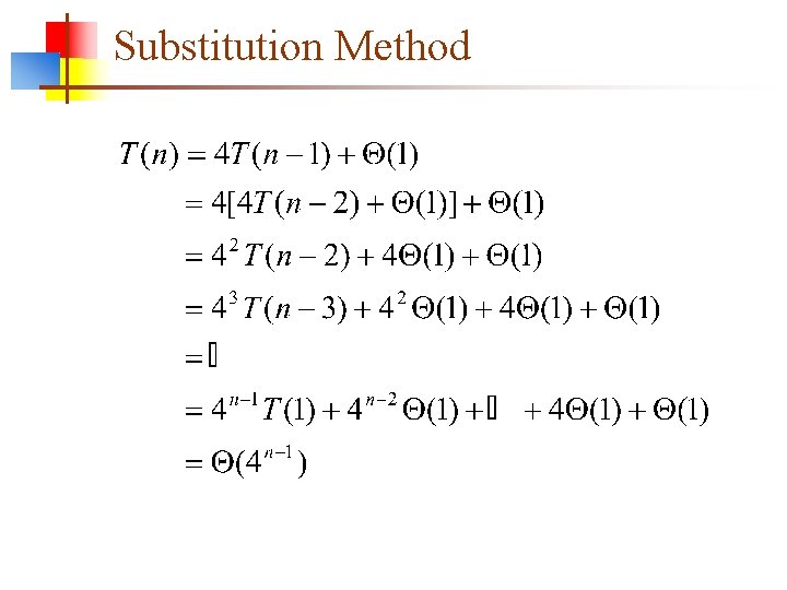
Complexity n n Let T(n) be the time taken to tile a 2 n× 2 n defective chessboard. T(0) = d, where d is a constant. T(n) = 4 T(n-1) + c, when n > 0. Here c is a constant. Recurrence equation

Substitution Method

Homework n Page 63 -65 5. 1 5. 3 5. 8 5. 10 5. 18 实验 5. 19 5. 21和5. 22至少选择 2题* 57