Dynamic Programming Nithya Tarek Dynamic Programming l l

Dynamic Programming Nithya Tarek

Dynamic Programming l l Dynamic programming solves problems by combining the solutions to sub problems. Paradigms: l l l Divide and conquer Greedy Algorithm Dynamic programming

String Matching l l Longest common subsequence Knuth-Morris-Pratt pattern matching

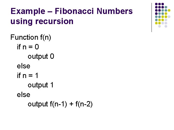
Example – Fibonacci Numbers using recursion Function f(n) if n = 0 output 0 else if n = 1 output 1 else output f(n-1) + f(n-2)

Example – Fibonacci Numbers using recursion l l Run time: T(n) = T(n-1) + T(n-2) This function grows as n grows The run time doubles as n grows and is order O(2 n). This is a bad algorithm as there are numerous repetitive calculations.

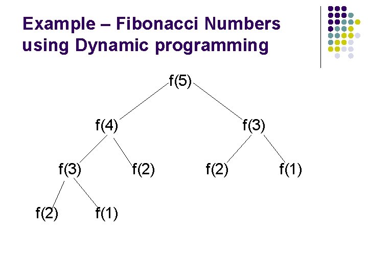
Example – Fibonacci Numbers using Dynamic programming f(5) f(4) f(3) f(2) f(1)

Example – Fibonacci Numbers using Dynamic programming l l l Dynamic programming calculates from bottom to top. Values are stored for later use. This reduces repetitive calculation.

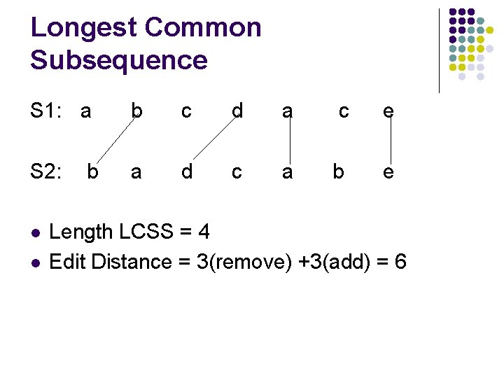
Longest Common Subsequence l l The input to this problem is two sequences S 1=abcdace and S 2=badcabe. The problem is to find the longest sequence that is a subsequence of both S 1 and S 2 where S 1 ≠ S 2. Distance between S 1 and S 2 is defined as the number of characters we have to remove from one string and add to that string to make S 1 and S 2 equal.

Longest Common Subsequence S 1: a b c d a c e S 2: a d c a b e l l b Length LCSS = 4 Edit Distance = 3(remove) +3(add) = 6

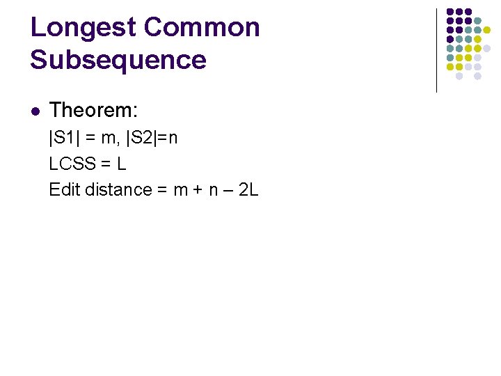
Longest Common Subsequence l Theorem: |S 1| = m, |S 2|=n LCSS = L Edit distance = m + n – 2 L

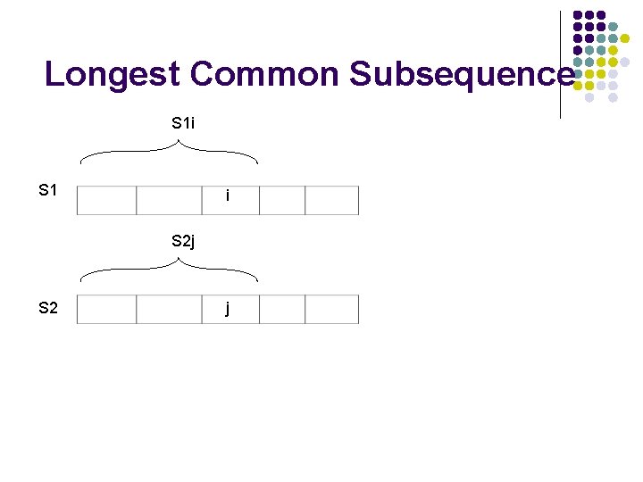
Longest Common Subsequence S 1 i S 1 i S 2 j S 2 j

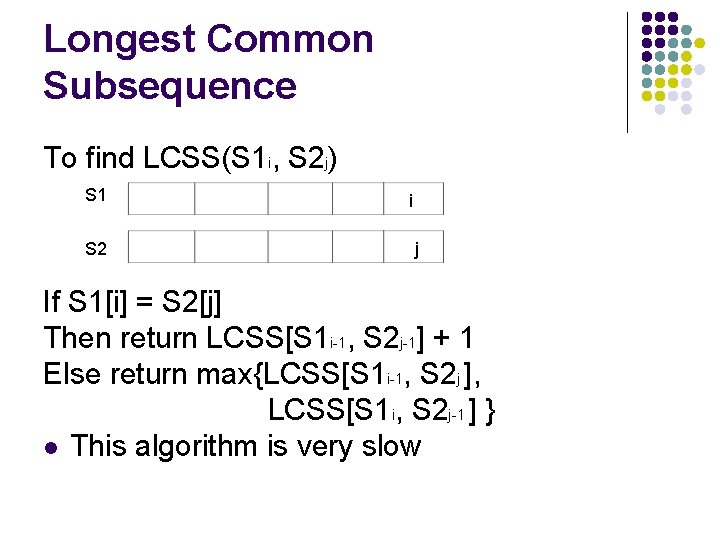
Longest Common Subsequence To find LCSS(S 1 i, S 2 j) S 1 S 2 i j If S 1[i] = S 2[j] Then return LCSS[S 1 i-1, S 2 j-1] + 1 Else return max{LCSS[S 1 i-1, S 2 j ], LCSS[S 1 i, S 2 j-1 ] } l This algorithm is very slow

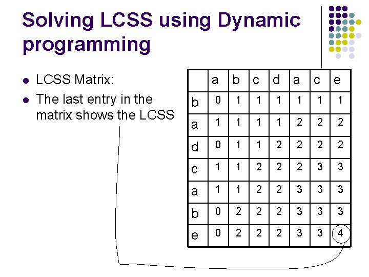
Solving LCSS using Dynamic programming l l LCSS Matrix: The last entry in the matrix shows the LCSS a b c d a c e b 0 1 1 1 a 1 1 2 2 2 d 0 1 1 2 2 c 1 1 2 2 2 3 3 a 1 1 2 2 3 3 3 b 0 2 2 2 3 3 3 e 0 2 2 2 3 3 4

Solving LCSS using Dynamic programming l l Runtime for this matrix using Dynamic programming is order of O(m, n) O(1) times to fill up each entry There are mn entries. Space required: O(mn)

Advantages of Dynamic programming l l A recursive procedure does not have memory Dynamic programming stores previous values to avoid multiple calculations

Space and Time l l The space can be reduced to order of O(min{m, n}) It is enough to keep only two rows j and j-1 After calculating the entries for row j move that row up to row j-1 and delete row j-1 and get the new entries for row j. The time cannot be reduced

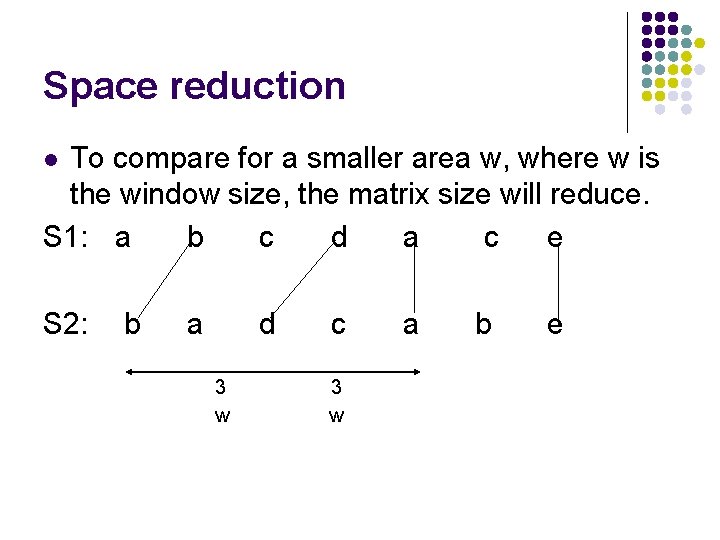
Space reduction To compare for a smaller area w, where w is the window size, the matrix size will reduce. S 1: a b c d a c e l S 2: b a d 3 w c 3 w a b e

Space reduction Specifying the window size reduces the number of calculation l The runtime of this algorithm is: O(2 w * min{m, n}) It is a linear time algorithm and the space required: O(w) l