Divide and Conquer Sorting Data Structures Insertion Sort

Divide and Conquer Sorting Data Structures

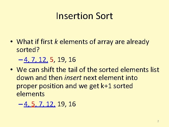
Insertion Sort • What if first k elements of array are already sorted? – 4, 7, 12, 5, 19, 16 • We can shift the tail of the sorted elements list down and then insert next element into proper position and we get k+1 sorted elements – 4, 5, 7, 12, 19, 16 2

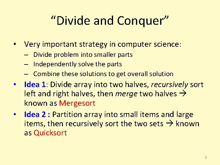
“Divide and Conquer” • Very important strategy in computer science: – Divide problem into smaller parts – Independently solve the parts – Combine these solutions to get overall solution • Idea 1: Divide array into two halves, recursively sort left and right halves, then merge two halves known as Mergesort • Idea 2 : Partition array into small items and large items, then recursively sort the two sets known as Quicksort 3

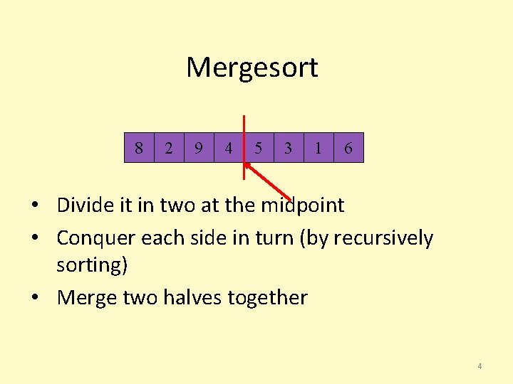
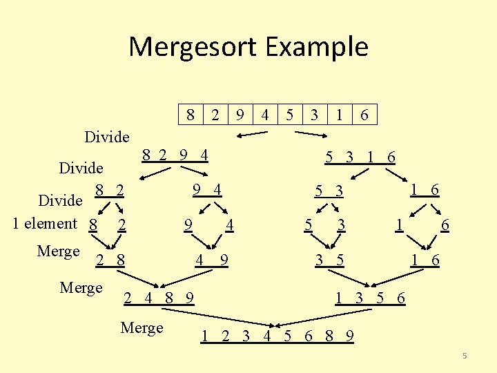
Mergesort 8 2 9 4 5 3 1 6 • Divide it in two at the midpoint • Conquer each side in turn (by recursively sorting) • Merge two halves together 4

Mergesort Example 8 Divide 8 2 Divide 1 element 8 2 Merge 9 4 5 3 8 2 9 4 9 2 4 8 9 Merge 6 1 6 5 3 4 4 1 5 3 1 6 9 4 2 8 Merge 2 9 5 3 1 3 5 6 1 2 3 4 5 6 8 9 5

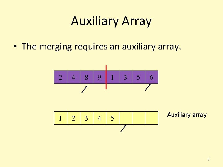
Auxiliary Array • The merging requires an auxiliary array. 2 4 8 9 1 3 5 6 Auxiliary array 6

Auxiliary Array • The merging requires an auxiliary array. 2 1 4 8 9 1 3 5 6 Auxiliary array 7

Auxiliary Array • The merging requires an auxiliary array. 2 4 8 9 1 1 2 3 4 5 3 5 6 Auxiliary array 8

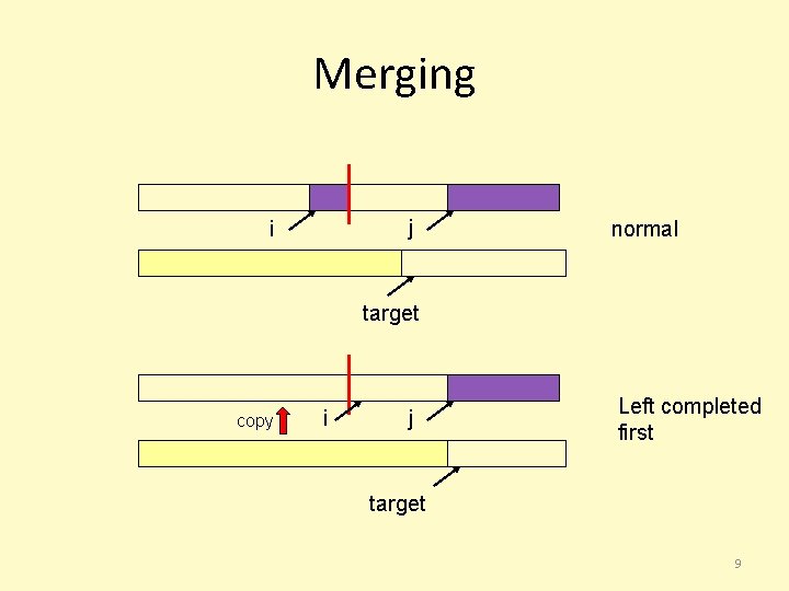
Merging j i normal target copy i j Left completed first target 9

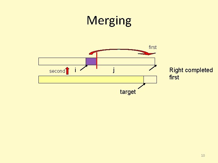
Merging first second i j Right completed first target 10

Merging Merge(A[], T[] : integer array, left, right : integer) : { mid, i, j, k, l, target : integer; mid : = (right + left)/2; i : = left; j : = mid + 1; target : = left; while i < mid and j < right do if A[i] < A[j] then T[target] : = A[i] ; i: = i + 1; else T[target] : = A[j]; j : = j + 1; target : = target + 1; if i > mid then //left completed// for k : = left to target-1 do A[k] : = T[k]; if j > right then //right completed// k : = mid; l : = right; while k > i do A[l] : = A[k]; k : = k-1; l : = l-1; for k : = left to target-1 do A[k] : = T[k]; } 11

Recursive Mergesort(A[], T[] : integer array, left, right : integer) : { if left < right then mid : = (left + right)/2; Mergesort(A, T, left, mid); Mergesort(A, T, mid+1, right); Merge(A, T, left, right); } Main. Mergesort(A[1. . n]: integer array, n : integer) : { T[1. . n]: integer array; Mergesort[A, T, 1, n]; } 12

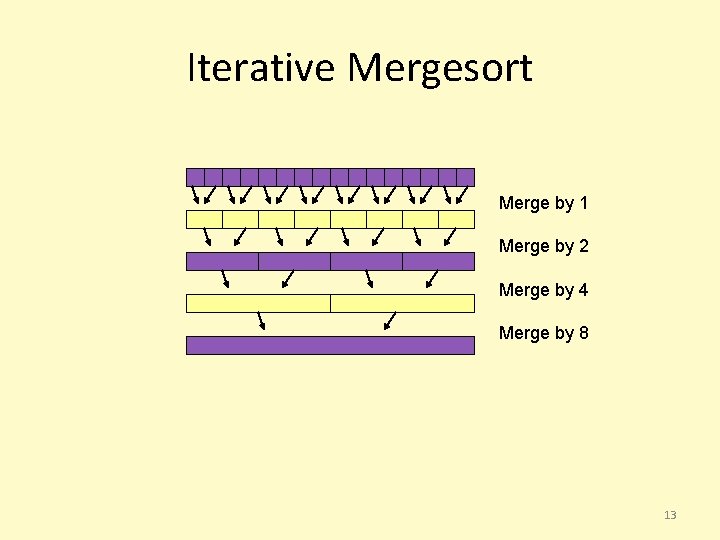
Iterative Mergesort Merge by 1 Merge by 2 Merge by 4 Merge by 8 13

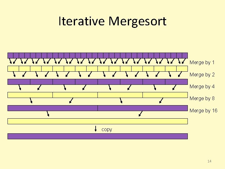
Iterative Mergesort Merge by 1 Merge by 2 Merge by 4 Merge by 8 Merge by 16 copy 14

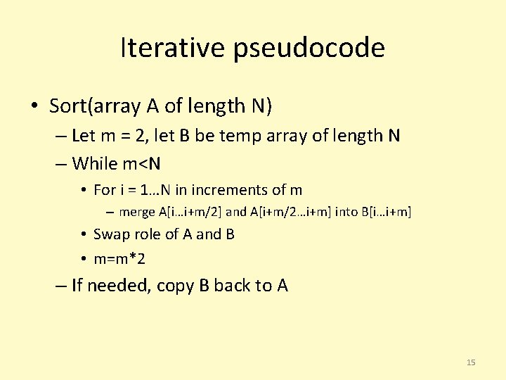
Iterative pseudocode • Sort(array A of length N) – Let m = 2, let B be temp array of length N – While m<N • For i = 1…N in increments of m – merge A[i…i+m/2] and A[i+m/2…i+m] into B[i…i+m] • Swap role of A and B • m=m*2 – If needed, copy B back to A 15

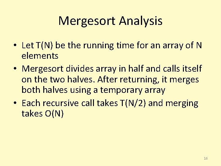
Mergesort Analysis • Let T(N) be the running time for an array of N elements • Mergesort divides array in half and calls itself on the two halves. After returning, it merges both halves using a temporary array • Each recursive call takes T(N/2) and merging takes O(N) 16

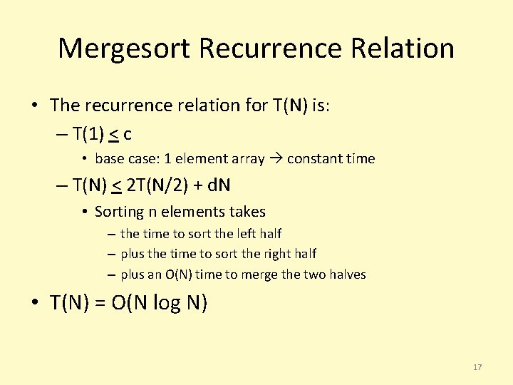
Mergesort Recurrence Relation • The recurrence relation for T(N) is: – T(1) < c • base case: 1 element array constant time – T(N) < 2 T(N/2) + d. N • Sorting n elements takes – the time to sort the left half – plus the time to sort the right half – plus an O(N) time to merge the two halves • T(N) = O(N log N) 17

Properties of Mergesort • Not in-place – Requires an auxiliary array • Very few comparisons • Iterative Mergesort reduces copying. 18

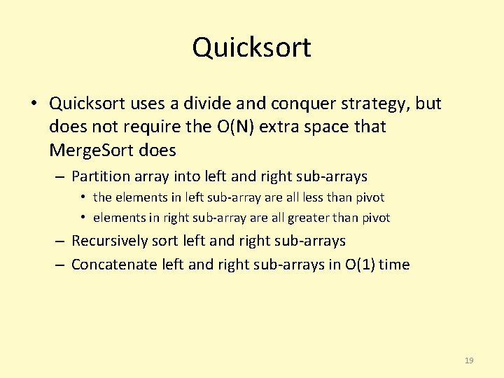
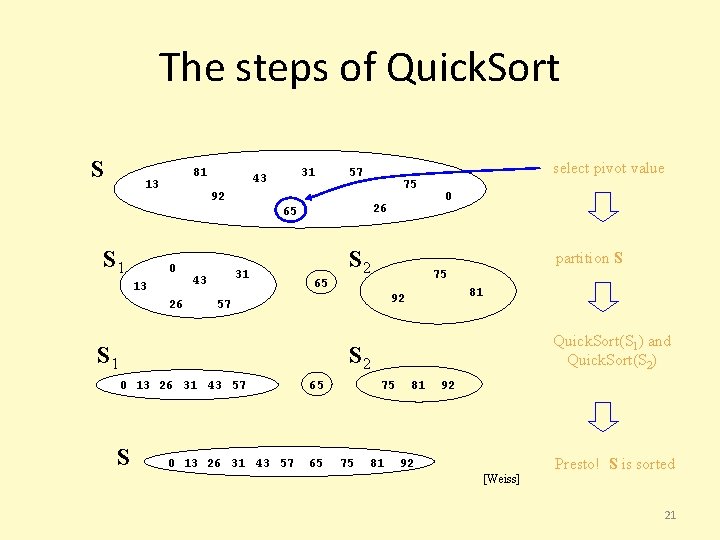
Quicksort • Quicksort uses a divide and conquer strategy, but does not require the O(N) extra space that Merge. Sort does – Partition array into left and right sub-arrays • the elements in left sub-array are all less than pivot • elements in right sub-array are all greater than pivot – Recursively sort left and right sub-arrays – Concatenate left and right sub-arrays in O(1) time 19

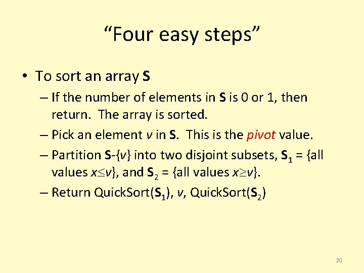
“Four easy steps” • To sort an array S – If the number of elements in S is 0 or 1, then return. The array is sorted. – Pick an element v in S. This is the pivot value. – Partition S-{v} into two disjoint subsets, S 1 = {all values x v}, and S 2 = {all values x v}. – Return Quick. Sort(S 1), v, Quick. Sort(S 2) 20

The steps of Quick. Sort S 81 13 31 43 select pivot value 57 75 92 26 65 S 1 0 13 26 31 43 S 2 0 partition S 75 65 81 92 57 S 1 Quick. Sort(S 1) and Quick. Sort(S 2) S 2 0 13 26 31 43 57 65 S 65 0 13 26 31 43 57 75 75 81 81 92 92 [Weiss] Presto! S is sorted 21

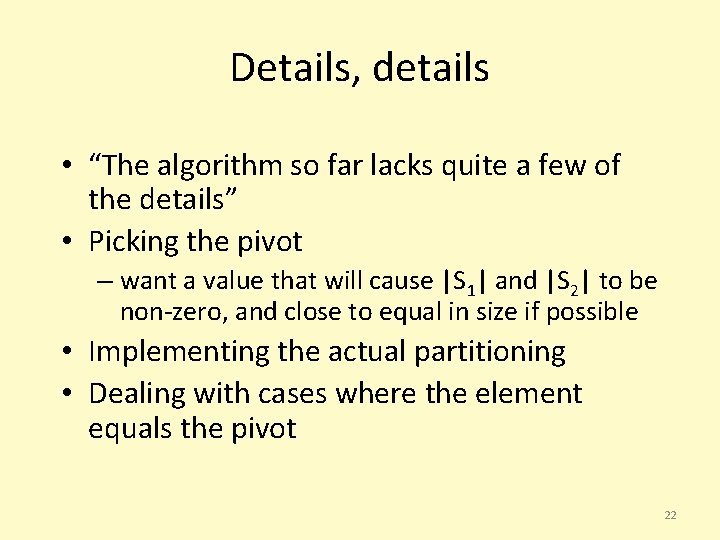
Details, details • “The algorithm so far lacks quite a few of the details” • Picking the pivot – want a value that will cause |S 1| and |S 2| to be non-zero, and close to equal in size if possible • Implementing the actual partitioning • Dealing with cases where the element equals the pivot 22

Alternative Pivot Rules • Chose A[left] – Fast, but too biased, enables worst-case • Chose A[random], left < random < right – Completely unbiased – Will cause relatively even split, but slow • Median of three, A[left], A[right], A[(left+right)/2] – The standard, tends to be unbiased, and does a little sorting on the side. 23

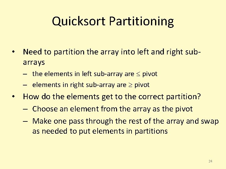
Quicksort Partitioning • Need to partition the array into left and right subarrays – the elements in left sub-array are pivot – elements in right sub-array are pivot • How do the elements get to the correct partition? – Choose an element from the array as the pivot – Make one pass through the rest of the array and swap as needed to put elements in partitions 24

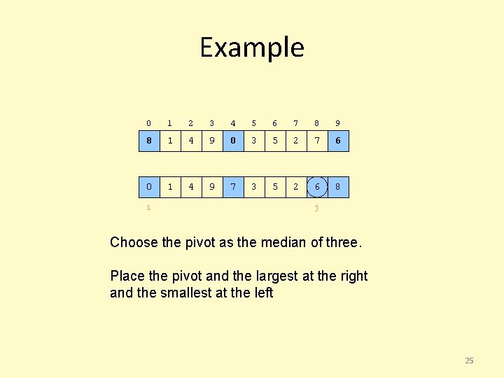
Example 0 1 2 3 4 5 6 7 8 9 8 1 4 9 0 3 5 2 7 6 0 1 4 9 7 3 5 2 6 8 i j Choose the pivot as the median of three. Place the pivot and the largest at the right and the smallest at the left 25

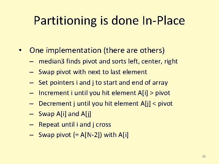
Partitioning is done In-Place • One implementation (there are others) – – – – median 3 finds pivot and sorts left, center, right Swap pivot with next to last element Set pointers i and j to start and end of array Increment i until you hit element A[i] > pivot Decrement j until you hit element A[j] < pivot Swap A[i] and A[j] Repeat until i and j cross Swap pivot (= A[N-2]) with A[i] 26

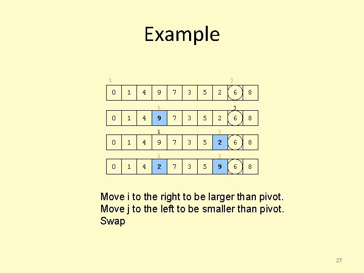
Example i 0 j 1 4 9 7 3 5 2 i 0 1 4 9 7 3 5 1 4 2 2 6 8 6 8 j 7 3 5 i 0 8 j i 0 6 2 j 7 3 5 9 Move i to the right to be larger than pivot. Move j to the left to be smaller than pivot. Swap 27

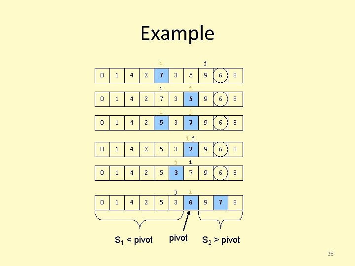
Example i 0 1 4 2 7 j 3 5 i 0 1 4 2 7 1 4 2 5 6 8 9 6 8 9 7 8 j 3 5 i 0 9 j 3 7 i j 0 0 0 1 1 1 4 4 4 2 2 2 S 1 < pivot 5 5 5 3 7 j i 3 6 pivot S 2 > pivot 28

Recursive Quicksort(A[]: integer array, left, right : integer): { pivotindex : integer; if left + CUTOFF right then pivot : = median 3(A, left, right); pivotindex : = Partition(A, left, right-1, pivot); Quicksort(A, left, pivotindex – 1); Quicksort(A, pivotindex + 1, right); else Insertionsort(A, left, right); } Don’t use quicksort for small arrays. CUTOFF = 10 is reasonable. 29

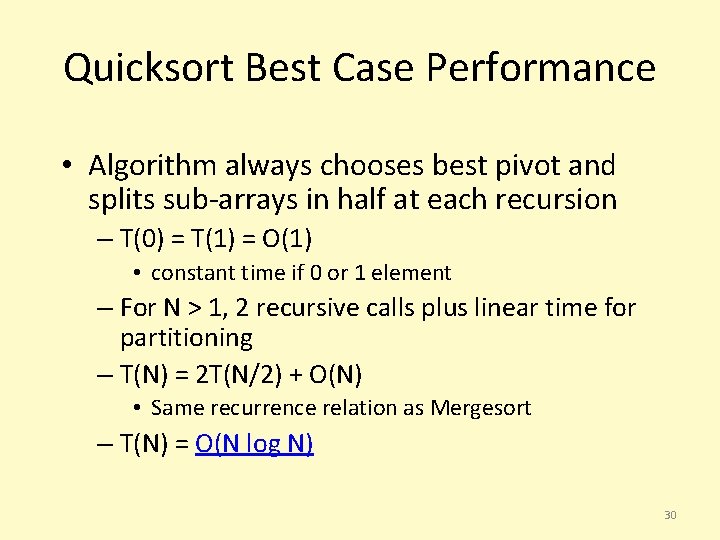
Quicksort Best Case Performance • Algorithm always chooses best pivot and splits sub-arrays in half at each recursion – T(0) = T(1) = O(1) • constant time if 0 or 1 element – For N > 1, 2 recursive calls plus linear time for partitioning – T(N) = 2 T(N/2) + O(N) • Same recurrence relation as Mergesort – T(N) = O(N log N) 30

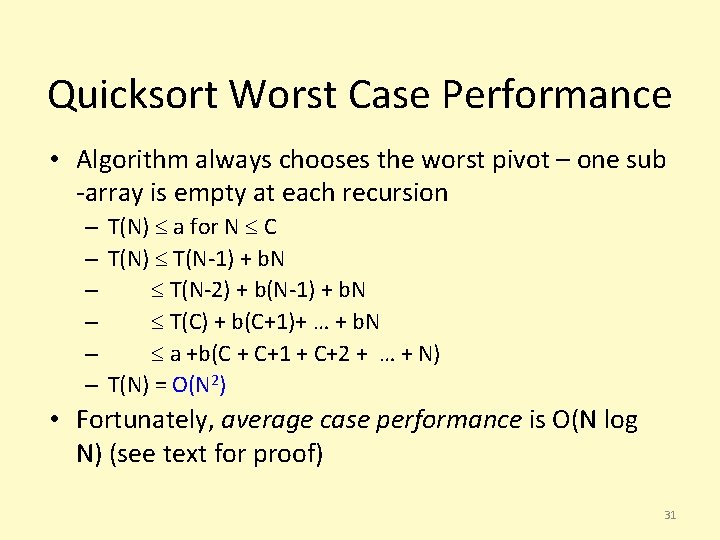
Quicksort Worst Case Performance • Algorithm always chooses the worst pivot – one sub -array is empty at each recursion – T(N) a for N C – T(N) T(N-1) + b. N – T(N-2) + b(N-1) + b. N – T(C) + b(C+1)+ … + b. N – a +b(C + C+1 + C+2 + … + N) – T(N) = O(N 2) • Fortunately, average case performance is O(N log N) (see text for proof) 31

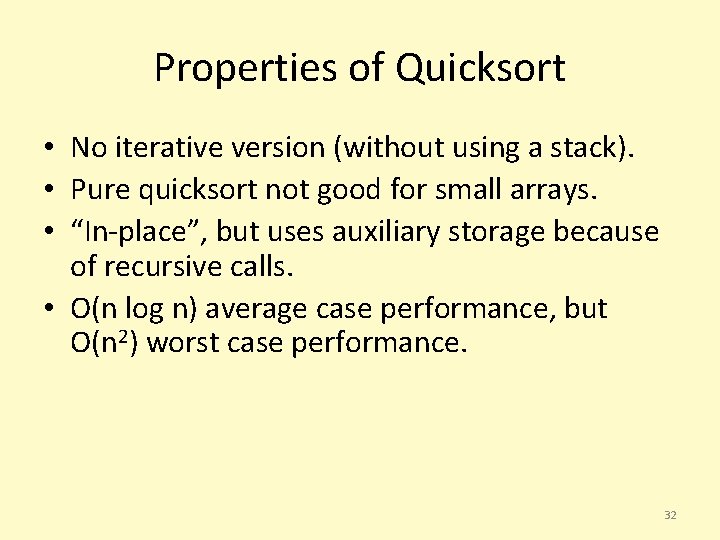
Properties of Quicksort • No iterative version (without using a stack). • Pure quicksort not good for small arrays. • “In-place”, but uses auxiliary storage because of recursive calls. • O(n log n) average case performance, but O(n 2) worst case performance. 32

Folklore • “Quicksort is the best in-memory sorting algorithm. ” • Mergesort and Quicksort make different tradeoffs regarding the cost of comparison and the cost of a swap 33

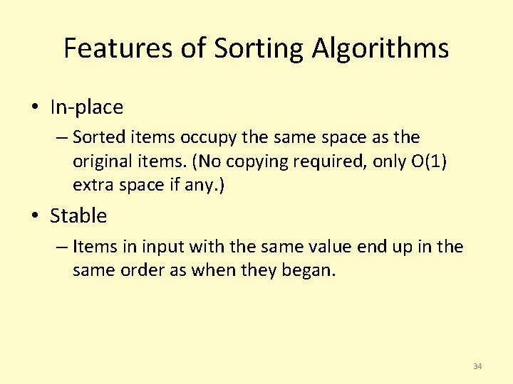
Features of Sorting Algorithms • In-place – Sorted items occupy the same space as the original items. (No copying required, only O(1) extra space if any. ) • Stable – Items in input with the same value end up in the same order as when they began. 34

How fast can we sort? • Heapsort, Mergesort, and Quicksort all run in O(N log N) best case running time • Can we do any better? • No, if the basic action is a comparison. 35

Sorting Model • Recall our basic assumption: we can only compare two elements at a time – we can only reduce the possible solution space by half each time we make a comparison • Suppose you are given N elements – Assume no duplicates • How many possible orderings can you get? – Example: a, b, c (N = 3) 36

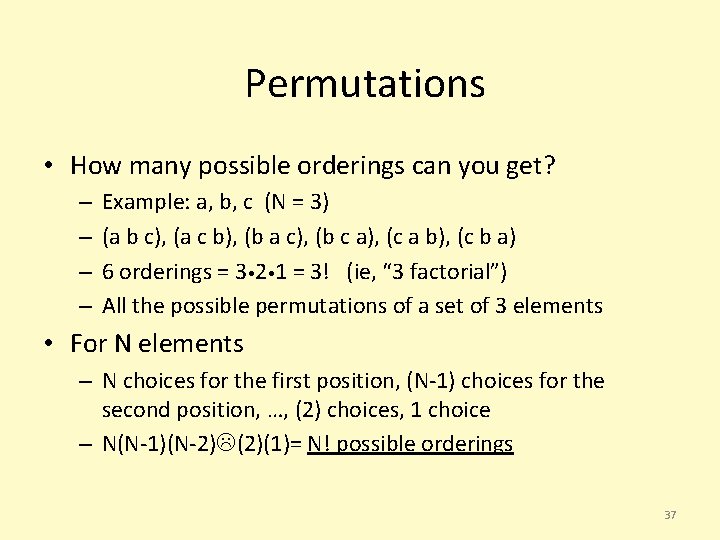
Permutations • How many possible orderings can you get? – – Example: a, b, c (N = 3) (a b c), (a c b), (b a c), (b c a), (c a b), (c b a) 6 orderings = 3 • 2 • 1 = 3! (ie, “ 3 factorial”) All the possible permutations of a set of 3 elements • For N elements – N choices for the first position, (N-1) choices for the second position, …, (2) choices, 1 choice – N(N-1)(N-2) (2)(1)= N! possible orderings 37

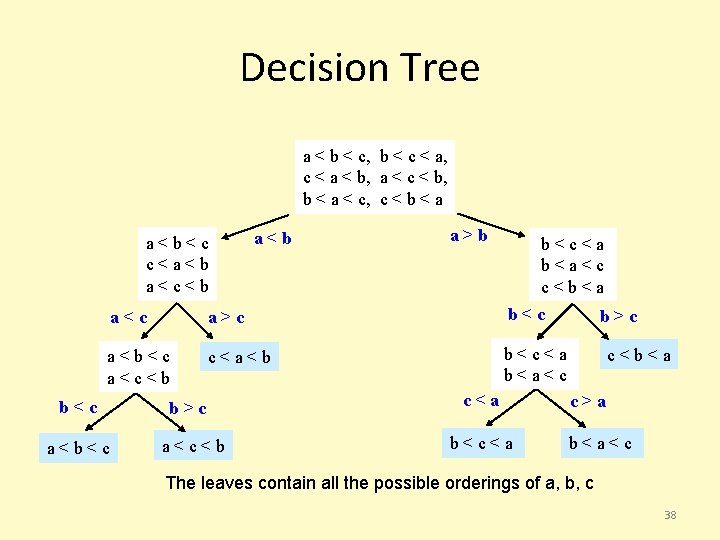
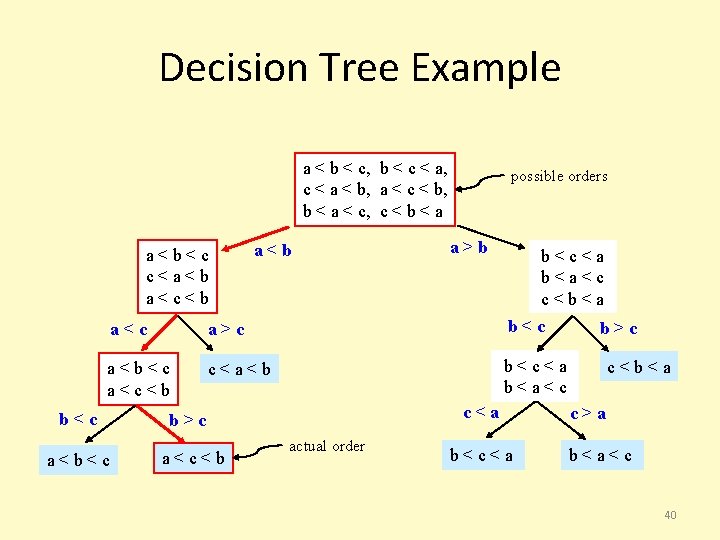
Decision Tree a < b < c, b < c < a, c < a < b, a < c < b, b < a < c, c < b < a a<b<c c<a<b a<c<b a>b b<c<a b<a<c c<b<a a<c a>c b<c a<c<b c<a<b b<c<a b<a<c b<c a<b<c b>c a<c<b c<a b<c<a b>c c<b<a c>a b<a<c The leaves contain all the possible orderings of a, b, c 38

Decision Trees • A Decision Tree is a Binary Tree such that: – Each node = a set of orderings • ie, the remaining solution space – Each edge = 1 comparison – Each leaf = 1 unique ordering – How many leaves for N distinct elements? • N!, ie, a leaf for each possible ordering • Only 1 leaf has the ordering that is the desired correctly sorted arrangement 39

Decision Tree Example a < b < c, b < c < a, c < a < b, a < c < b, b < a < c, c < b < a a<b<c c<a<b a<c<b a<b possible orders a>b b<c<a b<a<c c<b<a a<c a>c b<c a<c<b c<a<b b<c<a b<a<c b<c a<b<c c<a b>c a<c<b actual order b<c<a b>c c<b<a c>a b<a<c 40

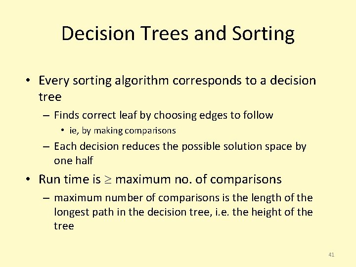
Decision Trees and Sorting • Every sorting algorithm corresponds to a decision tree – Finds correct leaf by choosing edges to follow • ie, by making comparisons – Each decision reduces the possible solution space by one half • Run time is maximum no. of comparisons – maximum number of comparisons is the length of the longest path in the decision tree, i. e. the height of the tree 41

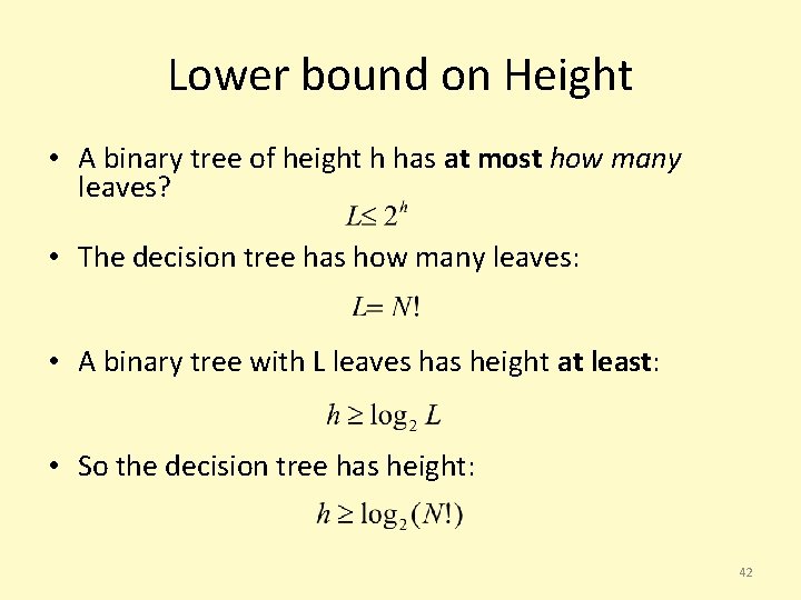
Lower bound on Height • A binary tree of height h has at most how many leaves? • The decision tree has how many leaves: • A binary tree with L leaves has height at least: • So the decision tree has height: 42

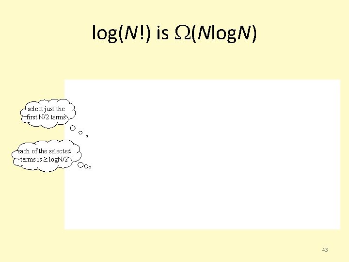
log(N!) is (Nlog. N) select just the first N/2 terms each of the selected terms is log. N/2 43

(N log N) • Run time of any comparison-based sorting algorithm is (N log N) • Can we do better if we don’t use comparisons? 44

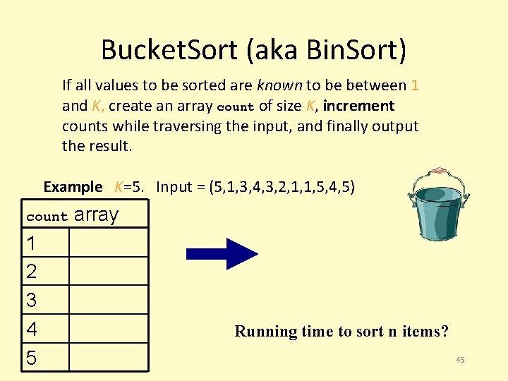
Bucket. Sort (aka Bin. Sort) If all values to be sorted are known to be between 1 and K, create an array count of size K, increment counts while traversing the input, and finally output the result. Example K=5. Input = (5, 1, 3, 4, 3, 2, 1, 1, 5, 4, 5) count 1 2 3 4 5 array Running time to sort n items? 45

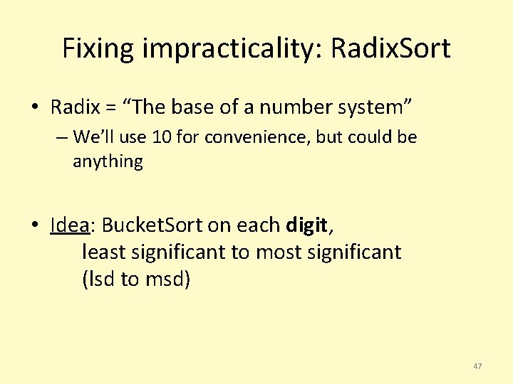
Bucket. Sort Complexity: O(n+K) • Case 1: K is a constant – Bin. Sort is linear time • Case 2: K is variable – Not simply linear time • Case 3: K is constant but large (e. g. 232) – ? ? ? 46

Fixing impracticality: Radix. Sort • Radix = “The base of a number system” – We’ll use 10 for convenience, but could be anything • Idea: Bucket. Sort on each digit, least significant to most significant (lsd to msd) 47

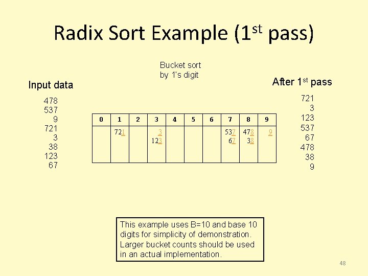
Radix Sort Example (1 st pass) Bucket sort by 1’s digit Input data 478 537 9 721 3 38 123 67 0 1 721 2 3 3 123 4 5 After 1 st pass 6 7 8 537 67 478 38 9 9 721 3 123 537 67 478 38 9 This example uses B=10 and base 10 digits for simplicity of demonstration. Larger bucket counts should be used in an actual implementation. 48

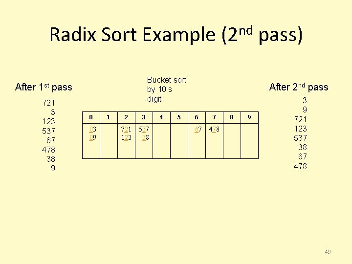
Radix Sort Example (2 nd pass) After 1 st Bucket sort by 10’s digit pass 721 3 123 537 67 478 38 9 0 03 09 1 2 3 721 123 537 38 4 5 After 2 nd pass 6 7 67 478 8 9 3 9 721 123 537 38 67 478 49

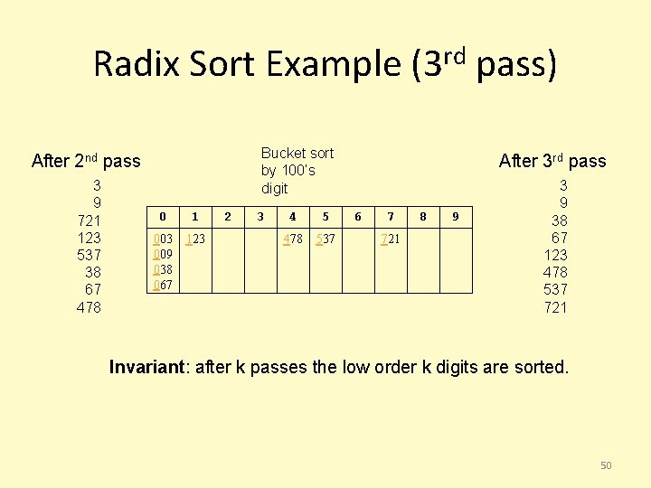
Radix Sort Example (3 rd pass) Bucket sort by 100’s digit After 2 nd pass 3 9 721 123 537 38 67 478 0 1 003 009 038 067 123 2 3 4 5 478 537 After 3 rd pass 6 7 721 8 9 38 67 123 478 537 721 Invariant: after k passes the low order k digits are sorted. 50

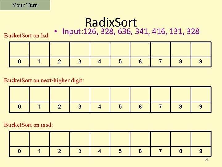
Your Turn Radix. Sort Bucket. Sort on lsd: 0 1 • Input: 126, 328, 636, 341, 416, 131, 328 2 3 4 5 6 7 8 9 Bucket. Sort on next-higher digit: 0 1 2 3 4 5 6 7 8 9 Bucket. Sort on msd: 0 1 51

Radixsort: Complexity • How many passes? • How much work per pass? • Total time? • Conclusion? • In practice – Radix. Sort only good for large number of elements with relatively small values – Hard on the cache compared to Merge. Sort/Quick. Sort 52

Summary of sorting • Sorting choices: – O(N 2) – Bubblesort, Insertion Sort – O(N log N) average case running time: • Heapsort: In-place, not stable. • Mergesort: O(N) extra space, stable. • Quicksort: claimed fastest in practice, but O(N 2) worst case. Needs extra storage for recursion. Not stable. – O(N) – Radix Sort: fast and stable. Not comparison based. Not in-place. 53